Why 4-Bit Weights Are Easy and 8-Bit Activations Break Models: Inside LLM Inference, Part 3

digitado ⋅ 2 de July de 2026

A systems-level mental model of quantization, built from the asymmetry that explains every method in the field

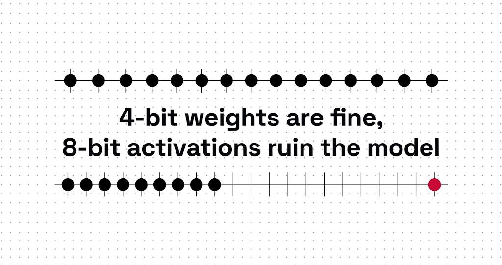
Quantizing the weights of a large language model is close to a solved problem. You can drop them from 16 bits to 4 bits and the behavior stays same. But quantizing the activations, the numbers flowing between layers, can destroy the same model completely, even at 8 bits. Even-though Both are just arrays of floating point numbers getting mapped onto a smaller grid, the outcome is not even close. Understanding why these two cases diverge so sharply is the foundation for reasoning about every quantization scheme you will ever encounter.

This is the third article in a series on the systems layer of LLM inference. The first and second established that decode is bound by memory bandwidth rather than compute, and that fact returns at the end of this one to explain when quantization actually makes a model faster.

The Asymmetry Nobody Tells You About
Outliers, the Few Numbers That Ruin Everything
How One Outlier Destroys a Whole Tensor
The Mapping Itself, Turning Floats Into Integers
Granularity, the Knob That Controls Everything
The Payoff in Bytes, VRAM Math From First Principles
Why Smaller Sometimes Means Faster, and Sometimes Doesn’t

1. The Asymmetry Nobody Tells You About

Most explanations of quantization treat it as one technique applied to one kind of number. You take a tensor, you compute a scale, you map the values onto a smaller integer grid. But there are two completely different tensors getting quantized inside a transformer, weights and activations, and they behave so differently that the same procedure succeeds on one and fails on the other. Every algorithm covered later in this series exists because of this split, so it is worth understanding precisely before anything else.

Two things get quantized, and they could not be more different

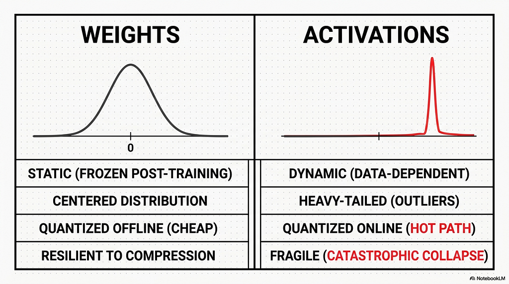
Weights are static. They are the parameters learned during training, and once training ends they are frozen. They do not change when the model runs. This means they can be analyzed exhaustively before deployment, with multi-pass profiling, grid searches over candidate scales, or second-order error minimization, none of which costs anything at inference time because the work happens once, offline, and the result is baked into the model file.

Activations are the opposite. They are the intermediate values computed during the forward pass, the outputs of matrix multiplications, normalization layers, and non-linear functions. They are data-dependent, so they change with every input token and every sequence the model processes. There is no fixed activation tensor to study ahead of time. Quantizing activations has to happen online, inside the inference hot path, while the model is generating tokens. This places a hard constraint on the method. Any scale factor or offset has to be cheap enough to compute on the fly, because expensive computation in the hot path directly reduces throughput. The clever offline tricks available for weights are mostly unavailable for activations, not because they would not work, but because there is no time to run them.

The shape of the numbers

The deeper problem is that weights and activations have completely different statistical shapes, and quantization is fundamentally about fitting a fixed grid to a distribution of values.

Pretrained transformer weights tend to follow stable, bell-shaped distributions clustered tightly around zero. They look roughly Gaussian. The range is bounded and predictable, which means a uniform grid of integer steps covers them well, with most of the grid’s resolution landing where most of the weights actually are. Mapping them onto a smaller integer range introduces little error because nothing is far from the center.

Activations in modern transformers do not behave this way. They tend to be heavy-tailed and are not centered on zero, and a small number of values sit enormously far from the rest. A grid that has to stretch far enough to cover those extreme values wastes almost all of its resolution on empty space, leaving the bulk of the distribution crushed into a handful of steps. The same uniform grid that fit the weights cleanly now represents the activations terribly.

The mechanism producing those extreme activation values, and why they are not random noise, is the subject of the next section. For now the load-bearing fact is that the difficulty does not come from the bit-width alone. It comes from the distribution the bits have to represent.

Why this one fact organizes everything that follows

This asymmetry is the spine of the entire topic. The distributions explain the outliers. The outliers explain why naive quantization collapses. The collapse explains why the field built an arsenal of algorithms, each one a different strategy for getting around the same problem. Reading the rest of this series through that chain, rather than as a list of separate techniques, is what makes a new and unfamiliar quantization scheme legible the first time you see it.

2. Outliers, the Few Numbers That Ruin Everything

The previous section established that activations are heavy-tailed and weights are not. That word, heavy-tailed, hides the actual problem. The tail is not a smooth gradual decline into larger values. It is a small number of specific values sitting orders of magnitude above everything around them, and they appear in predictable places. Understanding what these outliers are, and why a trained transformer produces them, is what makes the collapse in the next section inevitable rather than surprising.

What an outlier actually looks like

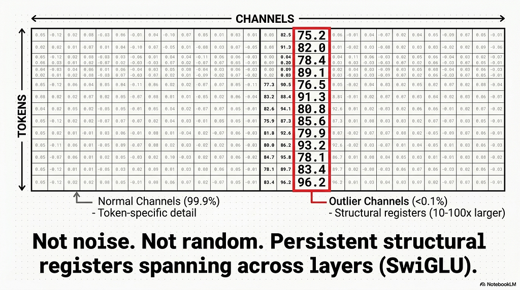
A typical activation outlier is between 10 and 100 times larger than the values surrounding it, and the channels carrying these outliers make up less than 0.1% of the total. Picture an activation tensor as a grid where each row is one token’s vector and each column is one channel. Most entries are small, sitting in a tight range near zero, the same well-behaved values that would quantize cleanly. Then one column holds values like 75 or 82 while its neighbors hold values like 0.1 or 0.05. That single column is the outlier channel, and it does not contain a stray large value in one token and normal values elsewhere. It is large for every token that passes through.

The persistence is the part that matters. If outliers were random spikes scattered across different channels for different tokens, they would average out and you could treat them as noise. They do not average out. The same channel index carries the extreme magnitude across token after token, across different input sequences, across different prompts entirely. Profiling the activations of a layer reveals the outlier channels sitting in fixed coordinate positions, and those positions stay put no matter what text the model is processing. This channel-wise pattern is the one that breaks quantization hardest, and it is the one this article follows. A separate token-wise variety also exists, where specific tokens rather than specific channels carry extreme magnitudes, but the channel-wise case is what drives the collapse traced here.

They are not noise, they are structure

This stability is what separates an outlier channel from measurement noise, and it is the property every algorithm later in this series exploits. A noisy spike cannot be planned around. A persistent structural feature can be. Because the outlier channels occupy known, fixed positions, a quantization method can isolate them, scale them, or route them through a separate path, all of which depend on the outliers staying where they were observed during calibration. The entire field of outlier-aware quantization rests on the fact that these channels are reliable rather than random.

The outliers also concentrate in specific parts of the network rather than spreading uniformly. In LLaMA-style architectures, the gating and down-projection paths of the SwiGLU feed-forward blocks produce particularly large activation magnitudes. The dynamic range of these activation vectors stretches by orders of magnitude relative to the weights feeding them, which is the precise mismatch that makes a single shared scale fail.

Where they come from

The outliers trace back to a specific limitation of the attention mechanism. The softmax inside attention cannot output an exact zero, because its exponential form always assigns some nonzero weight to every position. When an attention head needs to do almost nothing, effectively passing the residual stream through unchanged, it has to approximate that near-zero output by driving the inputs to the softmax to extreme magnitudes. Those extreme values then propagate into the activations elsewhere in the network. Research on quantizable transformers traced strong activation outliers directly to attention heads attempting this kind of no-op, where the pressure to produce near-zero attention weights pushes the pre-softmax values larger and larger during training.

The gated feed-forward blocks then amplify the effect, which is why the outliers concentrate where they do. In the SwiGLU blocks of LLaMA-style models, large responses in the gate and up-projection matrices get magnified by the SiLU activation and the gating multiplication, and further amplified in the down-projection, producing the persistent high-magnitude channels that profiling reveals. The values land in a small set of fixed coordinate dimensions because the mechanism that creates them is structural rather than input-dependent.

The practical consequence is that these channels cannot be discarded or clipped away without consequence. They are load-bearing. A quantization scheme that crushes them to fit a convenient grid is destroying information the model depends on to function, which is why naive approaches fail so completely.

3. How One Outlier Destroys a Whole Tensor

The previous section ended with a claim that needs to be shown rather than asserted, that a single outlier channel can drag an entire tensor down through nothing more than the arithmetic of a shared scale factor. This section traces that arithmetic step by step. The mechanism is simple enough to follow in three lines, which is exactly why it is dangerous. Nothing breaks, no error is thrown, the math runs as designed, and the model still produces garbage.

The single-scale trap

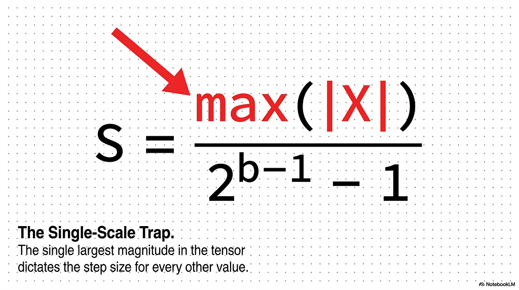
A per-tensor quantization scheme computes one scale factor for the whole tensor, and that scale is set by the largest absolute value present. The scale represents the real-world distance between two adjacent steps on the integer grid, and it has to be large enough that the most extreme value still lands inside the grid’s range. The formula is S = max(|X|) / (2^(b-1) – 1), where b is the target bit-width. The numerator is the single largest magnitude in the entire tensor. When that magnitude belongs to an outlier channel sitting 100 times above its neighbors, the outlier alone sets the step size for every other value in the tensor.

This is the trap. The scale factor does not care that 99.9% of the values are small and clustered. It only sees the maximum, and the maximum is an outlier. One channel that the model produced through the attention mechanism described in the previous section has now dictated the resolution of the entire grid.

The squeeze

A step size set by the outlier is far too coarse for the values that make up the bulk of the distribution. Consider an INT8 grid, which has 256 levels to work with. If the outlier stretches the scale so that one step equals a large jump in real value, then the small values, the ones sitting near zero where most of the activations live, all fall within the first one or two steps. They get rounded to the same handful of integers, or rounded to zero outright.

The values that get crushed are the ones carrying most of the model’s representational capacity. The normal channels encode the token-specific detail the model actually computes with, and quantization has just collapsed all of that detail into two or three indistinguishable levels. The outlier channel survives intact because the grid was built around it. Everything else is destroyed. The same failure gets sharper at INT4, where only 16 levels exist, so a stretched grid leaves the bulk of the distribution almost no resolution at all.

Why fully-quantized pipelines suffer most

The damage concentrates in pipelines that quantize both weights and activations to low precision at the same time, the configurations written as W8A8 and W4A4. The first number is the weight bit-width and the second is the activation bit-width, so W8A8 means 8-bit weights and 8-bit activations, and W4A4 pushes both to 4 bits.

These schemes force the activations, the tensors that carry the outliers, onto a restrictive grid with no high-precision path to fall back on. A weight-only scheme keeps the activations in FP16, which sidesteps the problem entirely because the outliers stay in a format wide enough to hold them. A fully-quantized scheme has no such escape. Both operands of the matrix multiplication sit on tight integer grids, and the activation grid is the one the outlier hijacks. This is why activation quantization is the hard problem and why so much engineering effort goes into it, while weight-only quantization remained close to solved.

The collapse traced here comes from using the most naive possible mapping, one scale, set by the raw maximum, applied uniformly. The next section steps back to the mapping operation itself and builds it up properly, starting with what a scale factor actually does and introducing the first real defense against the outlier problem, which turns out to be a matter of deciding where to put the edges of the grid.

4. The Mapping Itself, Turning Floats Into Integers

To understand why every real quantization method looks the way it does, the mapping operation itself has to be built up from the bottom, starting with what a scale factor represents and ending with the first technique that actually defends against outliers. Every method in the second half of this series is a variation on the primitive described here, so the payoff for getting it precise now compounds across everything that follows.

The core idea, a ruler with discrete ticks

Quantization maps a continuous range of floating point values onto a fixed set of integer slots, and the scale factor is the real-world distance between two adjacent slots. Think of laying a ruler over the range of values in a tensor. The ruler has a fixed number of ticks, 256 of them for INT8, 16 of them for INT4, and the scale is how much real value each tick is worth. A small scale means finely spaced ticks that resolve small differences. A large scale means coarsely spaced ticks that blur them together.

The forward operation takes a real value, divides it by the scale to find which tick it lands nearest, and rounds to that integer. Dequantization runs the same step backward, multiplying the stored integer by the scale to recover an approximation of the original. The error introduced is bounded by half a tick, because rounding can never push a value more than halfway to its neighbor. This is why the spacing matters so much. Coarse ticks mean large rounding error on every value they cover, which is precisely the damage the previous section traced when an outlier forced the spacing wide.

Symmetric and affine, and the zero-point

There are two ways to lay the ruler down, and they differ in whether the grid is forced to center on zero. Symmetric quantization centers the grid on zero, so the real value 0.0 maps to the integer 0, and the scale is set by the maximum absolute value in the tensor through s = max(|x|) / q_max. This is the scheme the previous section used. It is simple, it stores only a scale, and dequantization is a single multiply. But it assumes the values are roughly balanced around zero, and it wastes grid slots when they are not. A tensor whose values all sit between 0 and 10 would leave the entire negative half of a symmetric grid unused.

Affine quantization, also called asymmetric, fixes this by adding an integer zero-point offset. Rather than forcing real zero to integer zero, it shifts the grid so the actual minimum of the data maps to the bottom of the integer range and the actual maximum maps to the top. The zero-point is the integer that real zero maps to under this shift, and it is stored alongside the scale. This lets a skewed range use every available slot, which matters because activations after a function like ReLU are strictly non-negative, so a symmetric grid would waste its entire negative half on values that never occur.

The zero-point is not free. It adds a second parameter to store per scale, and it adds arithmetic to every dequantization, because recovering the real value now requires subtracting the offset before multiplying by the scale. The decision of whether to pay for affine quantization comes down to how skewed the distribution is. Weights, which are roughly symmetric around zero, gain little from a zero-point and usually use symmetric schemes. Activations, which are skewed, gain more and often justify the cost.

Absmax and its built-in weakness

Absmax quantization is the standard implementation of the symmetric scheme, and seeing it written out makes the earlier collapse exact rather than intuitive. The method takes the maximum absolute value in the tensor, maps it to the outermost tick of the integer grid, and sets the scale accordingly. Every other value falls proportionally inside that range. The appeal is that it preserves the relative magnitude of every element and requires nothing beyond a single max operation.

The weakness is now visible in the formula itself. Because the scale is max(|x|) / q_max, a single outlier in the numerator stretches the scale for the entire tensor. In a 4-bit or 8-bit grid, where there are few ticks to begin with, this stretching pushes the bulk of the distribution into the lowest one or two ticks, under-using the rest of the grid entirely.

Clipping, deliberately throwing away the tail

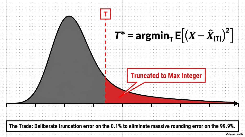
Clipping is the first real defense against outliers, and the idea is to stop letting the maximum value set the scale. Rather than mapping the true maximum to the edge of the grid, a clipping scheme picks a threshold T that sits below the true maximum, maps that threshold to the grid edge, and saturates everything above it to the maximum representable integer. The outliers get clipped to the ceiling. The bulk of the distribution, freed from having to share a grid stretched to accommodate the outlier, gets finely spaced ticks and low rounding error.

This is a deliberate trade. Clipping introduces truncation error on the handful of values above the threshold, in exchange for sharply reduced rounding error on the overwhelming majority below it. When 99.9% of the values are small and 0.1% are extreme, sacrificing precision on the 0.1% to gain it on the 99.9% is usually a favorable exchange. The open question is where to put the threshold, since too low destroys the outliers that the model needs and too high gives back the resolution that clipping was meant to recover.

The threshold is chosen by minimizing reconstruction error. The standard objective is to find the T that minimizes the mean squared error between the original values and their dequantized approximations, written as T* = argmin_T E[(X – X_hat(T))^2]. In practice the search is a grid search over candidate thresholds. For each candidate, the tensor is clipped, quantized, dequantized, and the resulting error is measured, and the threshold with the lowest error is kept.

The reason this works at no runtime cost traces directly back to the first section. Weights are static, so the entire grid search runs offline, once, before deployment, and the result is baked into the model. The expensive optimization happens where there is unlimited time to run it, and the inference path sees only the final scale. This is exactly the asymmetry that makes weight quantization tractable and activation quantization hard, the same asymmetry that opened the article, now showing up as the reason a technique like clipping is even available for weights.

Clipping treats the whole tensor with one threshold and one scale. The next refinement asks a different question, not where to put the grid edges, but how many separate grids to use in the first place.

5. Granularity, the Knob That Controls Everything

Everything in the previous section assumed one grid for the whole tensor, one scale, one threshold, one set of ticks covering every value. Granularity is the decision to use more than one. This is a separate axis from how each grid is built, because it asks how many independent scales to compute rather than where any single scale should sit, and it turns out to be the lever that most directly trades accuracy against storage in real quantization schemes. The configs you will encounter, the ones that say G=128 or per-channel or per-token, are all choices along this single axis.

The spectrum, from one scale to many

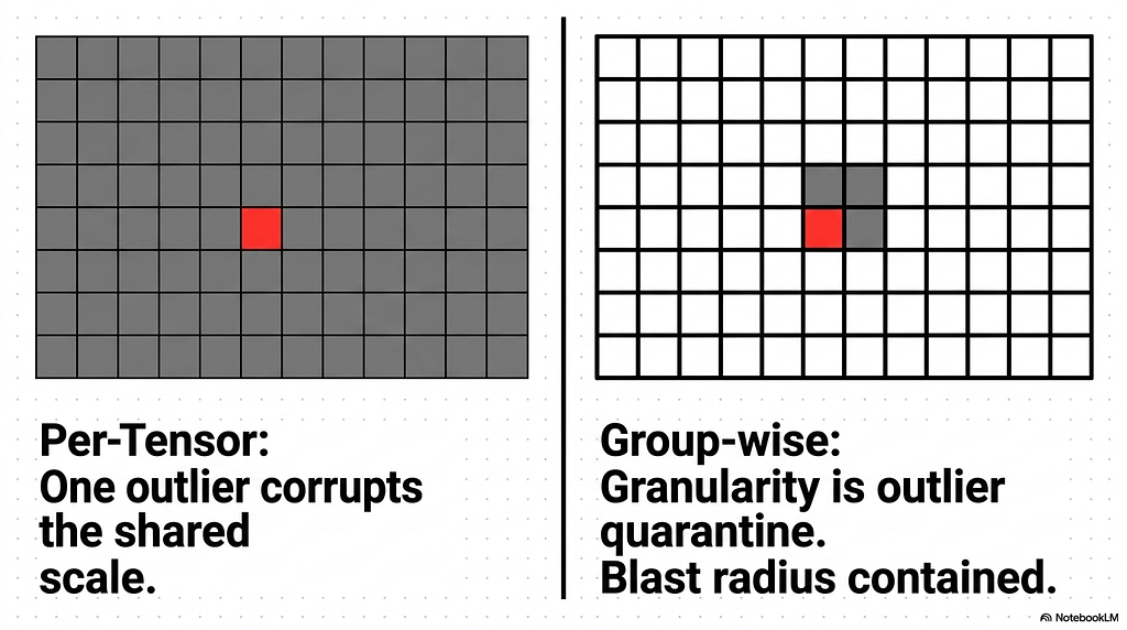
The coarsest option is per-tensor quantization, which computes a single scale for the entire multidimensional tensor. This is the scheme the third section collapsed. It stores the least metadata, one scale and optionally one zero-point for millions of values, and it is the most vulnerable to outliers because a single extreme value anywhere in the tensor sets the spacing for everything else.

Moving finer, the next options split the scales along a meaningful structural dimension. Per-channel quantization assigns one scale to each output channel of a weight matrix, so a row whose weights happen to be larger gets its own appropriately spaced grid rather than sharing one with a quieter row. Per-token quantization is the activation-side counterpart, computing a fresh scale for each individual token vector as it flows through the network, which handles the fact that different tokens produce activations of different magnitudes. Both of these adapt to structural variation while keeping the metadata cost low, because the number of channels or tokens is small relative to the number of values inside them.

The finest practical option is group-wise quantization, also called blockwise. This partitions the values along the reduction dimension into small contiguous blocks, typically 32, 64, or 128 elements each, and computes an independent scale for every block. A tensor of ten thousand values quantized with a group size of 128 gets roughly eighty separate scales, each covering its own narrow slice. The smaller the group, the more scales, and the more precisely each scale fits the values it covers.

The fundamental tradeoff

Smaller groups produce better accuracy and cost more metadata, and the relationship is direct enough to compute. Every scale factor is itself a number that has to be stored, usually in FP16, so the metadata overhead is the number of scales times their size. At a group size of 128 with 4-bit weights, the scales add roughly 3.125% to the stored size. At a group size of 64 the overhead doubles to about 6.25%, and at a group size of 32 it doubles again to about 12.5%. The accuracy climbs in the same direction, from good at 128 to near-lossless at 32, because each scale is responsible for fewer values and can fit them more tightly.

This is the tradeoff that the G number in a config name encodes. A scheme written as W4A16 with G=128 is making a specific bet, 4-bit weights with a scale every 128 elements, accepting about 3% metadata overhead in exchange for accuracy good enough that the bulk of the distribution quantizes cleanly. Choosing G=64 instead spends more memory to buy more fidelity. Reading a config means reading where on this spectrum its author chose to sit.

Why this connects to outliers

Granularity is an outlier-containment strategy, which is what ties it back to the problem the article has been building on since the second section. In a per-tensor scheme, one outlier corrupts the scale for the entire tensor, the collapse from the third section. In a group-wise scheme, that same outlier only corrupts the scale for its own block of 32 or 64 or 128 values. The damage is quarantined. The outlier still wastes the resolution of its block, but every other block in the tensor remains finely spaced and unaffected.

This reframes group size as a direct control on outlier blast radius. A smaller group means a smaller region that any single outlier can degrade, which is the deeper reason fine granularity recovers accuracy on the heavy-tailed distributions from the first section. The clipping from the fourth section decided how to handle outliers within one grid. Granularity decides how much of the tensor a single grid covers, and therefore how far the damage from any one outlier can spread.

The cost of all this finer granularity is the metadata, the scales that have to be stored and read alongside the quantized values. That cost has been described so far as a percentage, but percentages do not load models. The next section turns the entire picture into bytes.

6. The Payoff in Bytes, VRAM Math From First Principles

The previous section ended with metadata expressed as a percentage, and percentages are the wrong unit for the decision that actually matters, which is whether a given model fits on a given GPU. This section converts everything into bytes. The goal is a mental model precise enough to predict the memory footprint of any quantized model from three numbers, its parameter count, its bit-width, and its group size, and then to see why that footprint is often not the thing that decides whether the model runs.

Weight memory, the easy part

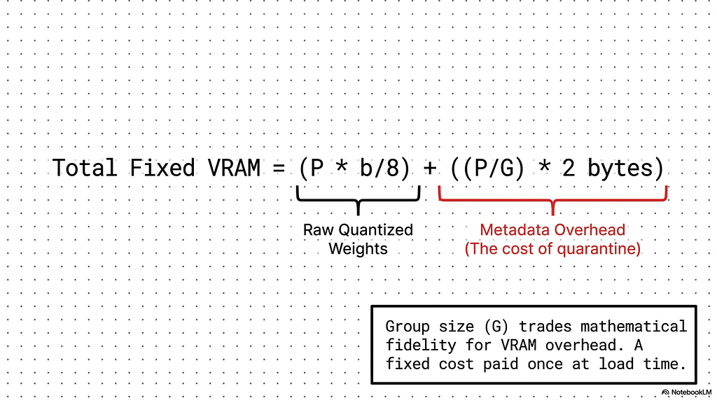
Weight memory is parameter count times bits per parameter divided by eight, and nothing about quantization changes the structure of that calculation. A model with P parameters stored at b bits per parameter occupies P * b / 8 bytes for its raw weights. An 8 billion parameter model in BF16, at 16 bits per parameter, needs roughly 16 GB. The same model quantized to 4 bits needs roughly 4 GB. The ratio is exactly the ratio of bit-widths, because the parameter count is fixed and only the per-parameter cost moves.

The one addition quantization makes is the metadata from the previous section, which has to be counted as real bytes rather than a percentage. Every group needs its scale stored, so a model with P parameters and group size G carries P / G scale factors, each typically an FP16 value at 2 bytes. For the 8 billion parameter model at 4-bit weights with a group size of 128, that is about 62.5 million scales at 2 bytes each, roughly 0.125 GB of metadata on top of the 4 GB of quantized weights. The scales add a few percent, exactly the overhead the previous section described, now in bytes that have to fit alongside everything else. Total weight memory is the raw quantized weights plus this metadata term, and for most consumer-facing quantization the metadata is small enough to treat as a minor correction rather than a dominant cost.

KV cache memory, the part that scales with usage

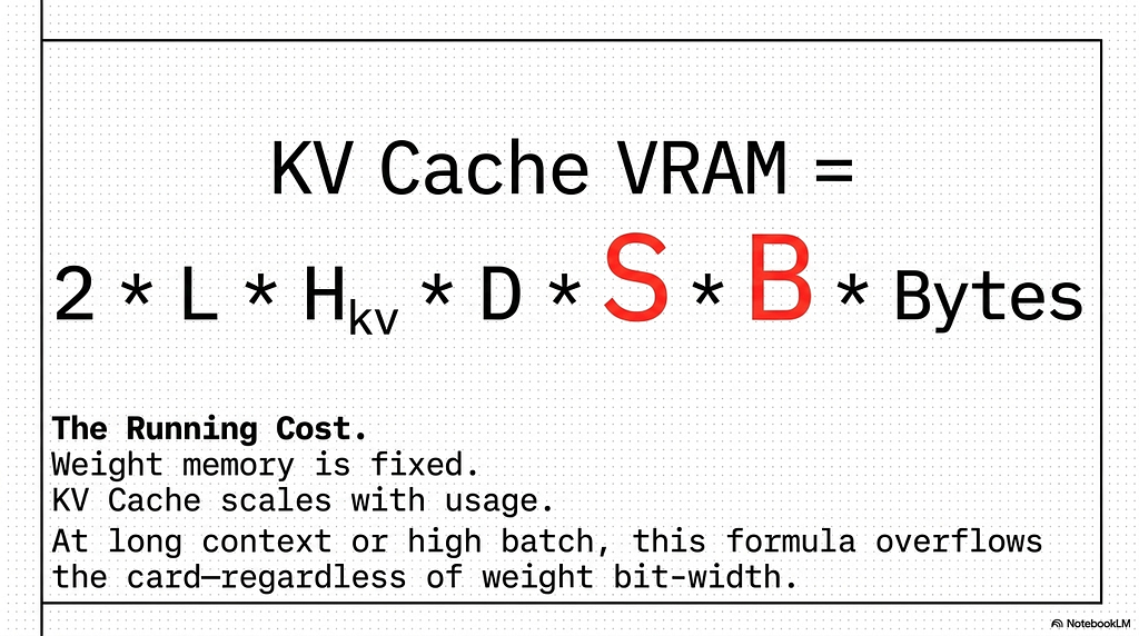
The KV cache is the memory that grows with how the model is used rather than how it was quantized, and it follows the same formula introduced in the first article of this series. For a model with L layers, H_kv key-value heads, head dimension D, processing a sequence of length S at batch size B, with each cached value taking bytes_per_element bytes, the cache occupies 2 * L * H_kv * D * S * B * bytes_per_element. The factor of two stores both the key and the value vectors. Nothing else gets cached, because every other intermediate is recomputed each step.

Grouped Query Attention is the architectural lever that shrinks this, and it does so by reducing H_kv directly. A model that uses 64 query heads but only 8 key-value heads stores keys and values for 8 heads rather than 64, an 8x reduction in cache size compared to giving every query head its own key-value pair. This is why the formula uses H_kv, the number of key-value heads, rather than the total attention head count, and it is the same H_kv that governed KV cache size in the bandwidth analysis of article one.

The reason the KV cache matters here is that it scales with batch size and sequence length while the weights do not. Weight memory is a fixed cost paid once when the model loads. KV cache is a running cost that climbs with every concurrent request and every additional token of context, and at long context or high batch it can grow past the weights entirely.

A worked scenario

Consider the 8 billion parameter model at 4-bit weights, group size 128, and compare its memory at two operating points. The weights are fixed at roughly 4 GB plus about 0.125 GB of scale metadata regardless of how the model is used. That is the entire static footprint, and it comfortably fits a consumer GPU.

Now add the KV cache at two batch sizes. The model has 32 layers, 8 key-value heads under GQA, and a head dimension of 128. At a sequence length of 8,192 tokens in FP16, one request’s cache is 2 * 32 * 8 * 128 * 8192 * 2 bytes, which works out to roughly 1 GB per request. At batch size 1, total memory sits near 5 GB, weights and cache together, and the weights dominate. At batch size 8, the cache becomes roughly 8 GB while the weights stay at 4 GB, and the running cost has overtaken the fixed cost. The model that fit easily at batch size 1 now needs more than twice the memory, and none of that growth came from the weights.

The lesson generalizes past this one model. Quantizing the weights shrinks the fixed cost, which is the cost most people focus on because it is the number on the model card, but it does nothing for the KV cache, which is frequently the cost that actually determines whether a workload fits. A reader sizing a deployment has to compute both terms, because halving the weights is irrelevant if the cache is what overflows the card. The same logic appears in production at scale, where a 70 billion parameter model at long context can demand more memory for its cache across a large batch than for its weights, regardless of how aggressively the weights were quantized.

Memory is only half of why quantization is worth doing. The other half is speed, and the relationship between the two is less direct than it appears, because a smaller model does not automatically run faster.

7. Why Smaller Sometimes Means Faster, and Sometimes Doesn’t

Memory math answers whether a model fits. It says nothing about whether the model runs faster, and those are different questions with different answers. A quantized model is smaller by definition, but smaller does not automatically mean faster, and understanding exactly when it does is what turns the preceding sections into a tool for reasoning about systems that have not been built yet. This is also where the gap from the opening of the article closes, the gap between knowing that quantization makes numbers smaller and knowing what that buys.

Decode is memory-bound

The first article in this series established the fact this section depends on, that LLM decode is bound by memory bandwidth rather than compute. Generating one token requires reading the entire set of model weights from high bandwidth memory, and the arithmetic performed against those weights is tiny relative to the bytes moved. The chip spends almost all of its time waiting for weights to arrive and almost none of it computing, which is why an FP16 decode workload on a large model can sit at a fraction of one percent of the chip’s peak compute. The binding constraint is how fast the weights can stream out of memory, not how fast the cores can multiply them.

Why weight-only quantization helps decode

Quantization speeds up decode by shrinking the exact thing that decode is bottlenecked on. Every decode step streams the full weight matrix from memory, so the time per token is set by the size of those weights divided by the memory bandwidth. Halve the bytes per weight, from 16-bit to 8-bit, and the bytes streamed per step halve, which halves the time per token at the same bandwidth. Drop to 4-bit and the streaming cost drops again. The speedup is close to linear in the bit-width reduction, and it comes entirely from moving fewer bytes.

The part worth holding onto is that this speedup happens even though the cores were already idle. The decode utilization derived in the first article sat near a third of a percent, meaning the compute units were doing almost nothing while waiting on memory. Quantization does not make them do more. It shortens the wait. The useful work per token stays the same, the time per token falls, and the throughput rises because the bottleneck resource, bandwidth, is now being asked to move less data. This is the reason quantization appears in essentially every production inference stack, and why cloud providers rarely serve full-precision weights, defaulting instead to quantized formats even on their most powerful hardware.

The catch

Weight-only quantization does not reduce the arithmetic, and this is where a naive implementation can erase the entire benefit. The hardware cannot multiply a 4-bit weight against a 16-bit activation directly, because standard accelerators do not perform mixed-precision matrix multiplication natively. The low-precision weights have to be converted back up to the activation’s format before the multiply happens. The math still runs in FP16. Only the storage and the streaming were ever in 4-bit.

A correct implementation does this conversion in the right place, streaming the compressed weights from memory into fast on-chip storage and expanding them to FP16 there, just before they enter the compute units, so the expanded high-precision version never travels across the slow memory bus. The bandwidth saving is preserved because the bytes that crossed the bottleneck were the small ones.

A naive implementation does it in the wrong place. It reads the compressed weights, expands them back to FP16, writes that expanded version back out to high bandwidth memory, and then reads it again to compute. The expanded weights now make the full trip across the memory bus at full FP16 size, which is the exact traffic quantization was supposed to avoid. The streaming cost returns to what it was before quantization, and the 4-bit model runs at the speed of the 16-bit model it replaced. This is the failure that explains why a 4-bit model can sometimes show no speedup at all, an implementation that pays the storage savings but throws away the bandwidth savings.

The mental model you can now apply

The question that predicts whether any quantization scheme speeds up any workload comes down to two parts. First, is the workload memory-bound, meaning is its runtime set by bytes moved rather than operations performed. Second, does the scheme actually reduce the bytes that cross the bottleneck. Both have to be true. A memory-bound workload whose quantization saves bytes runs faster. A compute-bound workload, like prefill or a very large batch, gains little from weight quantization because its bottleneck was never bandwidth in the first place, which is the same reason from article one that prefill saturates the cores while decode starves them.

This generalizes past quantization and past any specific system. Faced with a new optimization, a new chip, or a serving stack never seen before, the same two questions apply. Identify the bottleneck resource, then ask whether the technique reduces demand on that specific resource. A technique that shrinks something the workload was not bottlenecked on produces no speedup regardless of how impressive the compression ratio looks on paper.

Why 4-Bit Weights Are Easy and 8-Bit Activations Break Models: Inside LLM Inference, Part 3 was originally published in Towards AI on Medium, where people are continuing the conversation by highlighting and responding to this story.

Like 0

Liked Liked