")
Deep Learning Made Simple: What Neural Networks Actually Learn (Layer by Layer)

A visual, step-by-step guide using a cat vs dog classifier — with intuition, images, and Python code
Deep learning often feels like magic.
You feed an image of a cat into a model… and somehow it confidently says “cat”. But what actually happens inside the neural network?
What do layers really learn?
In this article, we’ll break it down in the simplest possible way — using a cat vs dog classification problem. You’ll see:
- What each layer in a neural network detects
- How raw pixels turn into meaningful features
- A visual intuition for every step
- A clean Python implementation
No heavy math. Just clear understanding.
Problem Setup: Cat vs Dog Classification
We want a model that takes an image like this:
And predicts:

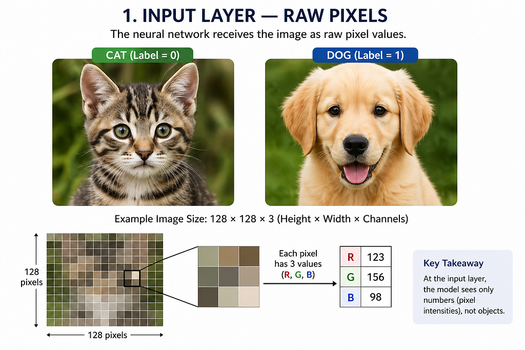
Step 1: The Input Layer — Raw Pixels
A computer does not see a “cat”.
It sees numbers.
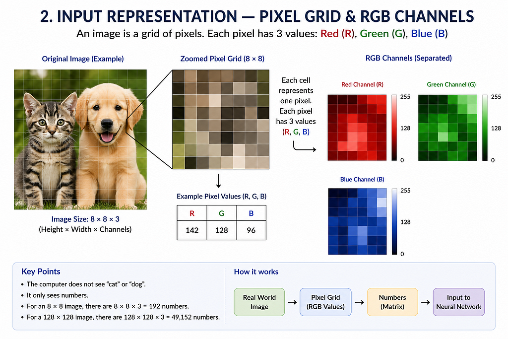
An image is just a grid:

Example:

Each pixel contains values between 0 and 255.
What the model sees:
At this stage:
- No understanding
- No shapes
- Just raw intensity values
Step 2: Convolution Layer — Detecting Edges
The first convolutional layer learns edges.
Edges are the foundation of vision.
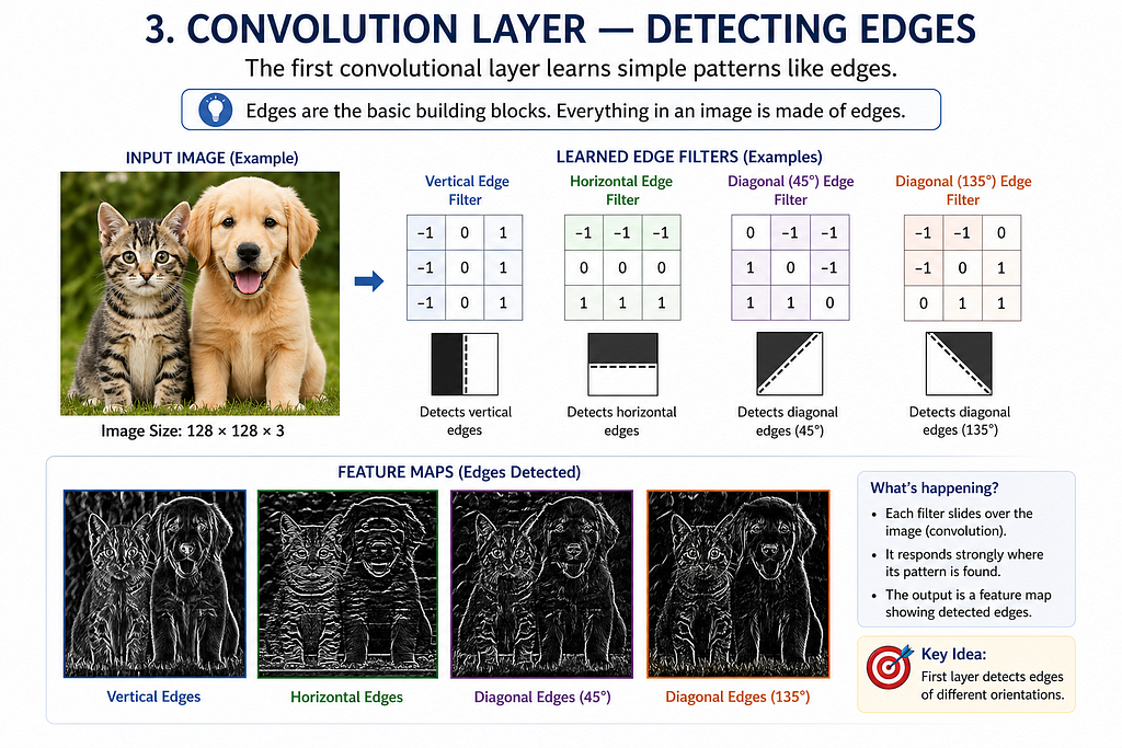
Typical filters detect:
- Vertical edges
- Horizontal edges
- Diagonal edges
Why edges?
Because everything (ears, eyes, tails) is built from edges.
Step 3: Activation Function (ReLU) — Adding Non-Linearity
After convolution, we apply an activation function like ReLU:

This removes negative values and keeps useful signals.
Effect:
- Keeps strong features
- Removes noise
Step 4: Pooling Layer — Reducing Complexity
Pooling reduces the image size while keeping important features.

Example:

Why pooling?
- Reduces computation
- Makes detection more robust to position changes
Step 5: Deeper Convolution Layers — Detecting Shapes
Now the network goes deeper.
Instead of edges, it starts detecting:
- Corners
- Curves
- Textures

At this level:
- The model starts recognizing parts of objects
Step 6: High-Level Layers — Detecting Object Parts
Deeper layers combine features into meaningful structures:
- Cat ears
- Dog snout
- Eyes
- Fur patterns
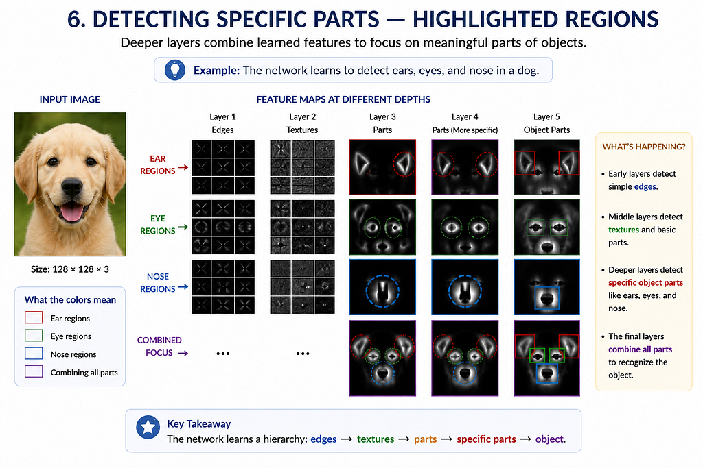
Now the model is no longer seeing pixels — it’s seeing semantics.
Step 7: Fully Connected Layer — Making the Decision
All extracted features are flattened and passed to dense layers.
These layers learn:
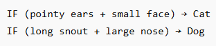
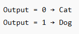
Step 8: Output Layer — Final Prediction
Final layer uses sigmoid activation:
Full Pipeline Overview


Python Implementation
Here’s a minimal working example using TensorFlow/Keras.
import tensorflow as tf
from tensorflow.keras import layers, models
import matplotlib.pyplot as plt

# Load dataset
(train_images, train_labels), (test_images, test_labels) = tf.keras.datasets.cifar10.load_data()

# Filter only cats (3) and dogs (5)
import numpy as np

train_filter = np.where((train_labels == 3) | (train_labels == 5))[0]
test_filter = np.where((test_labels == 3) | (test_labels == 5))[0]

train_images, train_labels = train_images[train_filter], train_labels[train_filter]
test_images, test_labels = test_images[test_filter], test_labels[test_filter]

# Convert labels: cat=0, dog=1
train_labels = (train_labels == 5).astype(int)
test_labels = (test_labels == 5).astype(int)

# Normalize
train_images = train_images / 255.0
test_images = test_images / 255.0

# Build model
model = models.Sequential([
    layers.Conv2D(32, (3,3), activation='relu', input_shape=(32,32,3)),
    layers.MaxPooling2D((2,2)),

    layers.Conv2D(64, (3,3), activation='relu'),
    layers.MaxPooling2D((2,2)),

    layers.Conv2D(64, (3,3), activation='relu'),
    layers.Flatten(),
    layers.Dense(64, activation='relu'),
    layers.Dense(1, activation='sigmoid')
])

# Compile
model.compile(optimizer='adam',
              loss='binary_crossentropy',
              metrics=['accuracy'])
# Train
history = model.fit(train_images, train_labels, epochs=5,
                    validation_data=(test_images, test_labels))

# Evaluate
test_loss, test_acc = model.evaluate(test_images, test_labels)
print("Test Accuracy:", test_acc)
Visualizing What the Model Learns
You can visualize intermediate layers:

This shows exactly what each layer is focusing on.
Python Implementation
import tensorflow as tf
import numpy as np
import matplotlib.pyplot as plt
from tensorflow.keras.datasets import cifar10

# Load data
(train_images, train_labels), _ = cifar10.load_data()

# Preprocess one image
img = train_images[0].astype("float32") / 255.0
img = np.expand_dims(img, axis=0)

# Define CNN (use your trained model here instead if available)
model = tf.keras.Sequential([
    tf.keras.layers.Conv2D(32, (3,3), activation='relu', input_shape=(32,32,3)),
    tf.keras.layers.MaxPooling2D((2,2)),
    tf.keras.layers.Conv2D(64, (3,3), activation='relu'),
    tf.keras.layers.MaxPooling2D((2,2)),
    tf.keras.layers.Conv2D(64, (3,3), activation='relu')
])

# Create model to output intermediate feature maps
layer_outputs = [layer.output for layer in model.layers if 'conv' in layer.name]
activation_model = tf.keras.Model(inputs=model.input, outputs=layer_outputs)

# Get feature maps
activations = activation_model.predict(img)

# Plot feature maps
for layer_idx, activation in enumerate(activations):
    num_filters = activation.shape[-1]
    size = activation.shape[1]

    cols = 8
    rows = num_filters // cols

    fig, axes = plt.subplots(rows, cols, figsize=(12, 12))
    fig.suptitle(f"Layer {layer_idx + 1} Feature Maps")

    for i in range(num_filters):
        r, c = divmod(i, cols)
        axes[r, c].imshow(activation[0, :, :, i], cmap='viridis')
        axes[r, c].axis('off')

    plt.show()
Figures and Tools Used
All figures were created by the author using Figma. The initial layout concepts and visual structuring were developed with AI-assisted guidance, followed by manual refinement and design implementation.
Final Thought
Deep learning is not magic.
It’s a hierarchy of simple transformations that gradually turn pixels into meaning.
Once you understand what each layer does, the entire field becomes far less mysterious — and far more powerful.
This article is based on established deep learning literature and widely used CNN architectures such as LeNet, AlexNet, and VGG-style networks
References
- Goodfellow, I., Bengio, Y., Courville, A. Deep Learning, MIT Press, 2016
- LeCun, Y. et al. (1998). Gradient-Based Learning Applied to Document Recognition
- Krizhevsky, A. et al. (2012). ImageNet Classification with Deep CNNs
- Zeiler, M., Fergus, R. (2014). Visualizing and Understanding Convolutional Networks
- Stanford CS231n: Convolutional Neural Networks for Visual Recognition
- TensorFlow Documentation: https://www.tensorflow.org/
Deep Learning Made Simple: What Neural Networks Actually Learn (Layer by Layer) was originally published in Towards AI on Medium, where people are continuing the conversation by highlighting and responding to this story.