
Deciphering the Complex Terms in Machine Learning (Gradient Based Optimization, Stochastic…
Deciphering the Complex Terms in Machine Learning (Gradient Based Optimization, Stochastic Objective Function Stochastic Gradient Descent Moments) — Part 1
In this story I am going to unravel few of the complex jargon terms we naturally face in machine learning papers In this study we are going to understand — Gradient Based Optimization, Stochastic Objective Function Stochastic Gradient Descent Moments used in Machine Learning.
i) First-order gradient-based optimization
A gradient tells us the direction in which a function increases fastest. In optimization, we usually want to minimize a loss function, so we move in the opposite direction of the gradient.
“First-order” means the algorithm uses only the first derivative, that is, the gradient.
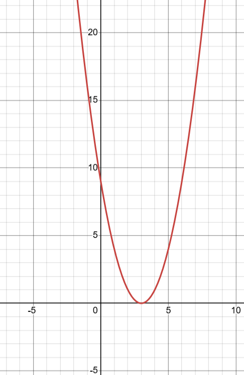
Suppose we want to minimize:
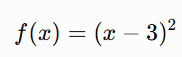
The minimum is clearly at x=3 since if we take any other values other than 3 we are not getting minimum values of f(x). To fully comprehend readers are required to workout the math and test different values.
The gradient is the first order derivative:
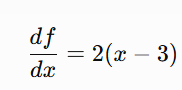
Since we are moving to the opposite direction of the increasing function, we are descending down the slope and that is why we call it gradient descent. we update the new gradient descent as:
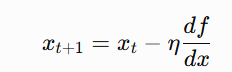
where η is the learning rate.
Example 1: One variable
Let:
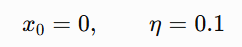
Gradient at x=0:
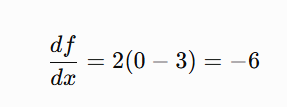
Now the Gradient Descent Update:
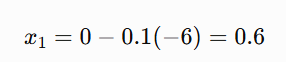
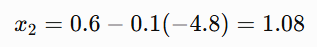
Next gradient:
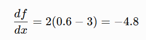
Update:
So x moves from:
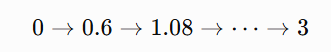
Example 2: Two variables
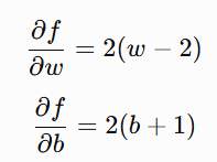
Suppose:
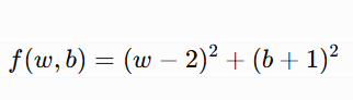
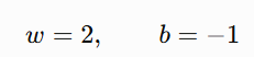
The minimum is at:
The gradients are Partial Derivative of each of the varibles:
Start from (suppose):
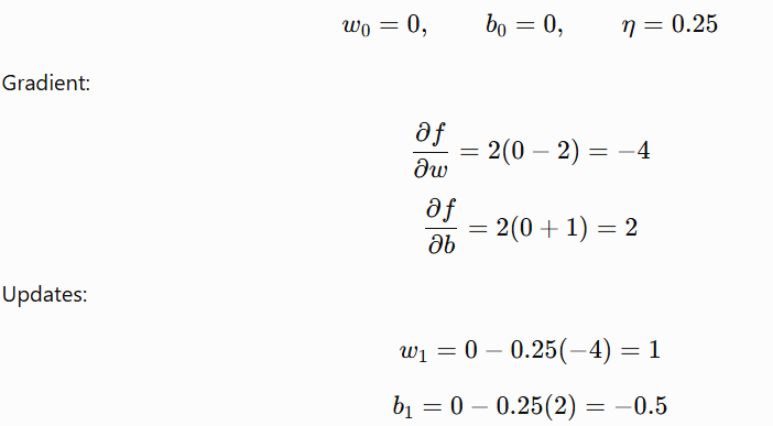
So the parameters move from:
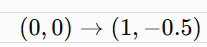
Again, they move closer to the minimum (2, -1)
A first-order optimizer uses gradients like these. It does not use second derivatives.
ii) Stochastic objective functions
A stochastic objective function is a loss function involving randomness.
In machine learning, we usually minimize an average loss:
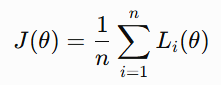
where:

represents model parameters, and Li(θ) is the loss from the i-th data point.
When the dataset is huge, calculating the gradient using all data points is expensive. So instead of using the full dataset every time, we use a small random batch. That makes the gradient stochastic or Probabilistic and here it means noisy but useful.
Example 1: Full objective
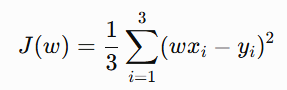
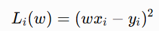
Suppose we have 3 data points so our objective function will be
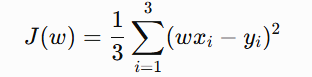
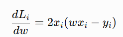
Differentiate both sides with respect to w:

Since 1/3 is a constant, it comes outside:
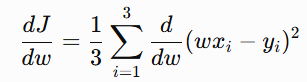
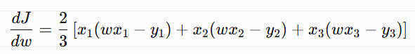
After applying the chain rule and completing the entire derivation we get:
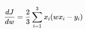
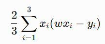
Suppose we have 3 data points (1,2), (2,4), (3,6) so:
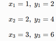
Since there are 3 data points:
At w = 0,
The gradient is:
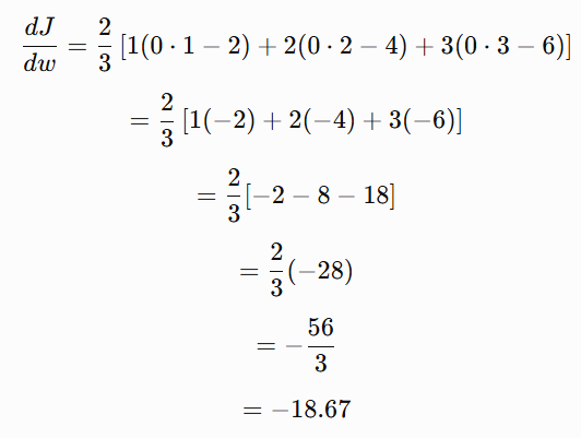
Therefore
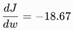
Meaning: at w=0, the loss decreases if we increase w, because the gradient is negative.
Example 2: Stochastic gradient using one random data point
Instead of all three points, suppose we randomly select only one point, so instead of using:
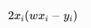
we randomly select one observation and use only its loss:
Its gradient is:
Notice the difference:
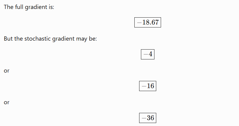
Full gradient:
Stochastic gradient for one point:
The stochastic gradient does not take the average over all three points. It uses only one selected point.
Case 1: Randomly selected point (1,2)
Here:
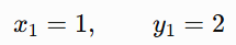
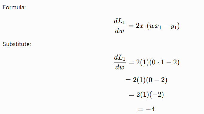
So if the selected point is (1,2), the stochastic gradient is -4.
Case 2: Randomly selected point (2,4)
Here:
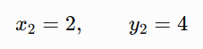
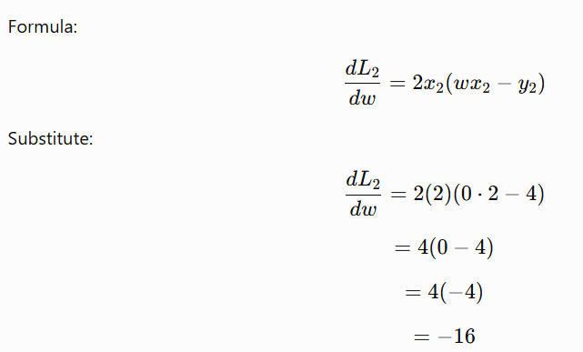
So if the selected point is (2,4) the stochastic gradient is: -16
Similarly if we take (3,6), the stochastic gradient is: -36
Why these are called noisy gradients
depending on which data point is randomly selected.
So instead of getting the exact full gradient -18.67 we get a noisy approximation: -4, -16, -36.
This is why it is called stochastic.
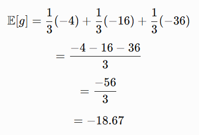
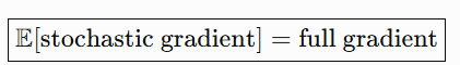
Important connection: average stochastic gradient equals full gradient
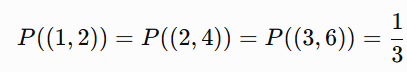
Since each point has equal probability of being selected:
Expected stochastic gradient:
iii) Moments
In statistics for a random variable X:
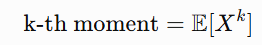
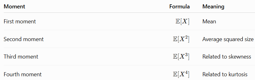
Lower-order moments usually mean the first and second moments.
Example 1: First moment
Suppose recent gradients are:
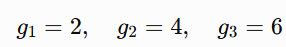
The first moment is the mean:
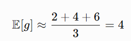
This tells the average direction of movement. For Adam optimizer, If the mean gradient is positive, Adam moves parameters downward. If the mean gradient is negative, Adam moves parameters upward.
Example 2: Second moment
Using the same gradients:
The second moment is:
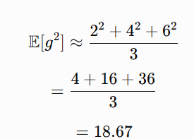
This tells Adam how large the gradients usually are.
Large second moment means: Big Gradient Activity and Small second moment means: Small Gradient Activity.
Example 3: Same mean, different second moment
Consider two gradient sequences:
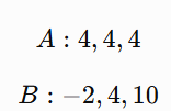
Both have mean:
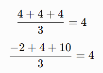
But their second moments are different.
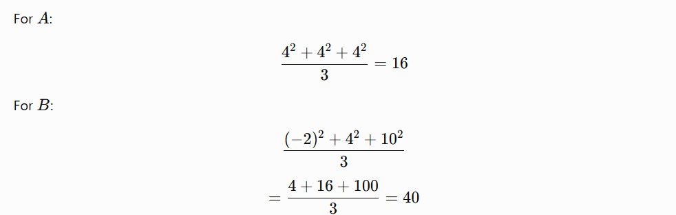
So although both have the same average direction, B has much larger gradient variation.
This is it for today’s discussion, I would love to hear some feedback. Thanak you.
Deciphering the Complex Terms in Machine Learning (Gradient Based Optimization, Stochastic… was originally published in Towards AI on Medium, where people are continuing the conversation by highlighting and responding to this story.