Optimizing Local LLM Inference on Constrained Hardware

digitado ⋅ 10 de June de 2026

An engineering deep dive into KV cache quantization, asymmetric thread tuning, and PCIe bottlenecks

Introduction

New frontier models launch weekly, and for most developers, the testing phase abruptly ends when the API bill arrives or the rate limit error appears. While proprietary models are the standard for rapid prototyping, they remain a black box. Users do not own the data, cannot strictly control latency, and are constrained by pricing tiers.

Local LLMs are the obvious alternative, offering privacy and zero recurring costs. However, for an engineer running inference on constrained hardware, the challenge isn’t just getting the model to run, it is optimizing how well it performs.

Recently, I transitioned my RAG and analytics pipelines to run locally on an older machine: an Intel i5–13450HX paired with a modest NVIDIA RTX 3050 (6GB VRAM). I initially chose Ollama for its ‘it just works’ appeal. But as context windows expanded, performance faltered. This led to an interesting hypothesis: the convenience of a high-level, Go-based wrapper was masking the true potential of the underlying hardware.

To reclaim performance, I bypassed the Ollama orchestration layer and interacted directly with llama.cpp. By manually tuning execution variables, managing direct memory addressing, and optimizing KV cache footprints, I achieved a ~100% performance increase on an 8-Billion parameter model.

This post details the raw benchmarks comparing high-level wrappers against bare-metal execution, and outlines the precise hardware tuning strategies required to maximize token generation on a strict 6GB VRAM budget.

The Mechanics of Local Inference: Understanding the Bottleneck

To optimize llama.cpp beyond its default configuration, we must understand the physical journey of a tensor. LLMs are auto-regressive, predicting the next token based on the sequence of all preceding tokens.

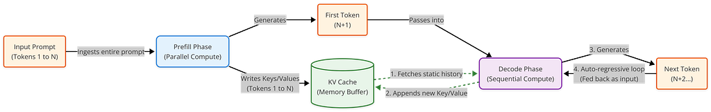
Every user request moves through two distinct, hardware-bound phases. Understanding which phase acts as the bottleneck is the prerequisite to optimization.

The Prefill Phase (Compute-Bound): During prefill, the model ingests the initial prompt and context. Because the entire prompt is known upfront, the engine processes the tokens in parallel. This phase is heavily reliant on raw computational power and is designed to fully saturate the GPU’s Tensor Cores.
The Decode Loop (Memory-Bandwidth Bound): This phase is where sequential generation of tokens takes place. Here, the bottleneck shifts entirely. The GPU is no longer limited by the mathematical operations per second, but by how fast it can fetch weights from the VRAM. For every single token generated, the engine must move the model’s weights from memory to the GPU cores. Therefore, Tokens Per Second (TPS) is primarily a function of memory bandwidth.

The KV Cache and the 6GB VRAM Wall

If an LLM had to reevaluate the entire context history to generate every single new token, the computational cost would scale quadratically, O(N²). To solve this, inference engines utilize a Key-Value (KV) Cache.

The KV Cache is a dedicated memory buffer in the VRAM that stores the computed hidden states (Keys and Values) of all previous tokens. Instead of reprocessing the entire history for every new word, the model fetches previous states from the cache and computes the math only for the single new token.

If your context is 100 tokens long and you want to predict token 101:

Without KV Cache: All 100 tokens are passed back into the transformer layers. The model re-calculates the Key (K) and Value (V) transformations for tokens 1 through 99 all over again, just to see how token 100 relates to them
With KV Cache: The K and V tensors for tokens 1 through 99 never change. They are static historical properties of those tokens within this context. By storing them in VRAM (the KV Cache), we only feed the single latest token into the model network.

The size of the KV cache scales linearly with context length and can be calculated using the formula.

For a Llama 3.1 8B model with a 16,000 token context window at standard FP16 precision, the exact memory overhead is as follows:

Model Weights (Q4_K_M): ~4.50 GB
KV Cache (16k context @ FP16): ~2.15 GB
Total Required VRAM: ~6.65 GB

This is where the physical limitations of a 6GB RTX 3050 become an impassable wall. When an orchestrator hits this ceiling, the system either crashes with an Out-Of-Memory (OOM) error or begins swapping the cache to system RAM. The moment tensor data spills over the PCIe bus into CPU memory, performance collapses.

Quantifying the “Abstraction Tax”

The local LLM ecosystem is heavily bifurcated: GUI-focused wrappers (like Ollama and LM Studio) versus high-throughput core engines (like vLLM and llama.cpp).

Written in Go, Ollama wraps llama.cpp, manages model distribution via a Docker-like manifest system, and provides a clean REST API. It abstracts away the friction of deployment. However, on a heavily constrained hardware budget, this abstraction introduces a “tax.”

To quantify this tax, I ran head-to-head benchmarks comparing Ollama against bare-metal execution via llama-cli (compiled natively with CUDA support DGGML_CUDA=ON). I tested three distinct real-world engineering scenarios and three different models:

Models :

Llama 3.2 3B: Fits entirely in VRAM
Llama 3.1 8B: A tight VRAM fit sitting exactly on the 6GB boundary
Mistral 24B: Massively oversized; forces a severe CPU/GPU split

Scenarios :

Simple QA (128 token prompt): Basic architectural Q&A
Coding Logic (512 token prompt): Writing optimized, tiled matrix multiplications
Long Context (16384 token prompt): Ingesting and summarizing Chapter 4 of the EU AI Act

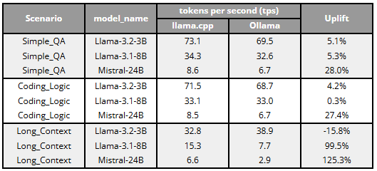
Performance Results (Tokens Per Second)

Llama 3.2 3B (Full VRAM Fit): When a model easily fits entirely inside the 6GB boundary, the abstraction tax is minimal. For short Q&A and medium coding logic, llama.cpp provided only marginal gains (~4–5% uplift, reaching ~73 TPS). Interestingly, during the Long Context scenario, Ollama actually outperformed llama.cpp execution by 15.8% (38.9 vs. 32.8 TPS). This suggests that when VRAM is abundant, high-level wrappers are highly optimized to handle standard context scaling out-of-the-box.
Llama 3.1 8B (The Edge of Capacity): Performance between the two engines was virtually identical for short and medium contexts (hovering around 33–34 TPS). However, the “abstraction tax” became glaringly obvious during the Long Context scenario. As the KV cache ballooned, Ollama conservatively spilled data into system RAM to prevent a crash, tanking performance to 7.7 TPS. By manually tuning llama.cpp, I forced those critical layers to remain in VRAM, yielding a 99.5% uplift (15.3 TPS).
Mistral 24B (Heavy CPU/GPU Split): Because this model vastly exceeds the 6GB limit, weights must constantly travel across the PCIe bus. Here, bare-metal execution dominated across the board. llama.cpp provided a steady ~28% uplift for short and medium prompts, but delivered a staggering 125.3% uplift (6.6 vs. 2.9 TPS) in the Long Context scenario. This proves that when memory bandwidth is severely bottlenecked, the overhead of a Go-based orchestration layer drastically amplifies PCIe latency.

The 8B Threshold and Conservative Scheduling

The 99.5% performance leap on the 8B model highlights the fundamental difference in memory management. When a model sits on the edge of VRAM capacity, high-level wrappers act conservatively to prevent crashes. Ollama offloads fewer layers to the GPU than the hardware can physically handle, preemptively spilling into the slow PCIe lane. By using llama.cpp directly, I manually forced the GPU to retain critical layers in VRAM, yielding double the throughput.

The PCIe Wall

When a model is massively oversized, standard orchestrators like Ollama struggle to manage the massive PCIe traffic, causing throughput to collapse to a nearly unusable 2.9 TPS. By switching to llama.cpp, we can streamline how memory is addressed across the CPU/GPU split, rescuing performance with a 125% uplift-proving that the heavier the hardware bottleneck, the more bare-metal tuning matters.

Advanced Optimization Strategies for llama.cpp

To understand how low-level configurations affect performance boundaries, I ran extensive benchmarking sweeps using llama-bench. Below are the empirical findings and the exact tuning parameters required to maximize hardware efficiency.

CPU Thread Optimization (-t): The Asymmetric Topology Trap

When a model (like Mistral 24B) exceeds VRAM, the CPU must shoulder the workload. On modern asymmetric processors (like the Intel i5–13450HX), simply maxing out the thread count usually degrades performance.

./build/bin/llama-bench 
  -m models/Mistral-Small-24B-Instruct-2501-Q2_K.gguf 
  -ngl 12 
  -fa 1 
  -p 512 
  -n 128 
  -t 4,6,8,10,12 
  -o csv > thread_optimization.csv

My benchmarks showed a clear prefill performance peak at 10 threads (263.9 tokens/s). Pushing execution to 12 caused prefill speeds to drop to 217.9 tokens/s.

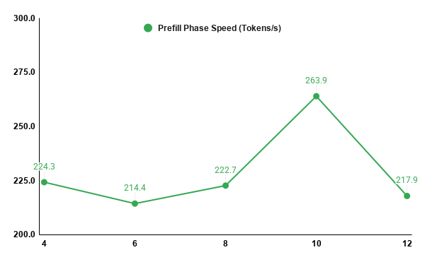
Why? The i5–13450HX features 6 Performance cores and 4 Efficiency cores (10 total physical cores). Allocating threads beyond the physical core count forces the fast P-cores to idle while waiting for the slower E-cores to complete synchronized matrix multiplications.

The Takeaway: Match your -t flag strictly to your physical core count. Ignore logical hyper-threading for LLM inference.

KV Cache Quantization Symmetry (-ctk / -ctv)

As context grows, compressing the KV cache is the only way to avoid an OOM crash on a 6GB card. However, the compression architecture matters immensely. I tested cache precision scaling from 16-bit float (f16) down to 4-bit quantization (q4_0).

./build/bin/llama-bench 
  -m models/Meta-Llama-3.1-8B-Instruct-Q4_K_M.gguf 
  -ngl 24 
  -fa 1 
  -p 4096 
  -n 128 
  -ctk f16,q8_0,q4_0 
  -ctv f16,q8_0,q4_0 
  -o csv > kv_cache_tradeoff.csv

The data revealed that mismatched precision formats (e.g., an f16 Key cache with a q4_0 Value cache) introduces a massive architectural penalty. Mixed precision breaks the optimized processing paths in llama.cpp, forcing the engine to perform format conversions mid-execution and collapsing prefill speeds to just 33.4 tokens/s.

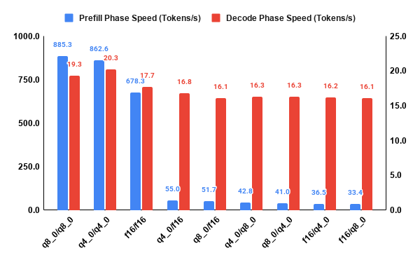
Conversely, using symmetric quantization (e.g., q4_0 for both Key and Value) routes data through highly optimized kernels. This reduced memory-bus congestion, increased token generation speed from 17.7 to 20.3 tokens/s, and slashed the cache’s VRAM footprint by nearly 75%.

The GPU Layer Offload Cliff (-ngl)

Offloading splits the model’s layers between the GPU and CPU. Because LLM layers process sequentially, intermediate tensors must constantly traverse the PCIe bus.

./build/bin/llama-bench 
  -m models/Meta-Llama-3.1-8B-Instruct-Q4_K_M.gguf 
  -fa 1 
  -p 512 
  -n 128 
  -ngl 0,8,16,24,32 
  -o csv > ngl_test_8b.csv

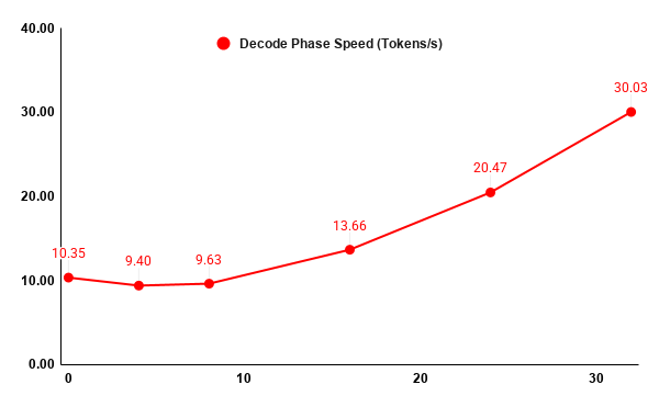
Benchmarking revealed a distinct performance trough. Moving from pure CPU execution (0 layers) to light hybrid offloading (4 to 8 layers) actually decreased decode performance (from 10.3 to 9.4 tokens/s). The overhead of moving intermediate tensors across the PCIe bus costs more time than the computational acceleration gained from the GPU. Performance only begins to scale positively once more than 50% of the layers (16+ layers) are offloaded.

The Takeaway: Offload all layers, or almost none. If you cannot fit a significant portion of the model in VRAM, the PCIe latency penalty will render your GPU effectively useless.

Batch vs. Micro-Batch Ingestion (-b vs -ub)

By adjusting batch sizes, we can tune how the GPU ingests massive blocks of text to prevent the “Warmup Spike”, a scenario where transient memory allocations crash the GPU driver.

I ran parameter sweeps altering the total batch size (-b) versus the physical micro-batch chunks (-ub) fed into the GPU.

./build/bin/llama-bench 
  -m models/Meta-Llama-3.1-8B-Instruct-Q4_K_M.gguf 
  -ngl 24 
  -fa 1 
  -p 1024 
  -n 128 
  -b 512,2048 
  -ub 128,512 
  -o csv > batch_size_evaluation.csv

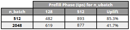
Increasing the micro-batch size (-ub) from 128 to 512 massively increased prefill speed by up to +85%. However, because it forces the GPU to process larger tensor chunks simultaneously, it requires more available VRAM padding to prevent an OOM crash. Decode speed remained entirely unaffected. This proves that micro-batch tuning is the single most effective lever for optimizing RAG pipelines (which are heavily prefill-dependent) on constrained hardware.

Conclusion

High-level wrappers like Ollama are incredible tools for velocity, prioritizing stability and ease of deployment. However, velocity often comes at the direct cost of hardware efficiency.

For data scientists and engineers operating on the edge, whether utilizing an aging 6GB gaming laptop or a constrained IoT device, defaults are usually the enemy. The “abstraction tax” is real, but entirely manageable. By dropping down to the bare metal, managing asymmetric CPU threads, symmetrically quantizing the KV cache, and understanding PCIe transfer limits, it is possible to double the throughput of standard local models.

When hardware is scarce, stripping away the orchestration layer transforms an underpowered machine from a struggling testing environment into a highly responsive inference engine.

All raw automated benchmarking scripts, configuration files, and datasets used to generate these profiles are open source and available in my GitHub repository.

Optimizing Local LLM Inference on Constrained Hardware was originally published in Towards AI on Medium, where people are continuing the conversation by highlighting and responding to this story.

Like 0

Liked Liked