: HNSW, IVF, BM25, Hybrid Search and Re-Ranking | M011 |…")
How RAG Actually Finds Answers (Part 2): HNSW, IVF, BM25, Hybrid Search and Re-Ranking | M011 |…
How RAG Actually Finds Answers (Part 2): HNSW, IVF, BM25, Hybrid Search and Re-Ranking | M011 | Mehul Ligade
🔴 Part 2 of a 3-Part RAG Series
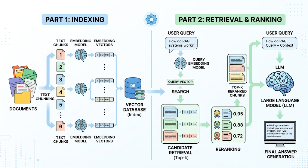
In Part 1, we built the mental model. We saw how PDFs become chunks, how chunks become embeddings, and how embeddings get stored inside a vector database so an AI system can search them later. That was the foundation.
Now we go one layer deeper and ask the real question: once the knowledge is already stored, how does the system actually find the right answer quickly and reliably? That is what this article is about. FAISS (Facebook AI Similarity Search) is one of the clearest references for this space because it is designed for efficient similarity search and clustering of dense vectors at scale, including datasets that may not fit in RAM.
🔴 The Real Retrieval Problem
Let us continue with the AI study assistant from Part 1. Imagine it contains thousands of lecture PDFs, textbook chapters, revision notes, and past exam papers. A student asks, “Explain gradient descent in simple words.” At first, this sounds easy. But under the hood, the system has to search through a huge number of chunks and choose the ones that truly matter. LangChain describes a retriever as an interface that takes an unstructured query and returns documents, which is a good way to think about this step: the system is not “thinking” yet, it is searching.
If the system simply compares the query with every stored vector one by one, the result is accurate but painfully slow at scale. That works for small prototypes. It does not work when the knowledge base grows into tens of thousands or millions of vectors.
This is why real retrieval systems depend on Approximate Nearest Neighbor, or ANN, search. ANN methods trade a tiny amount of exactness for a huge gain in speed, which is why they are so common in modern vector search stacks.
🔴 Approximate Nearest Neighbor Search
ANN is the idea of searching smart instead of searching everywhere. Rather than comparing the query against every vector in the database, the system uses an index that narrows the search space to the most promising candidates. Meta’s FAISS exists precisely for this reason: it is a library for efficient similarity search and clustering of dense vectors, and its documentation emphasizes that it supports very large-scale vector collections.
Two of the most important ANN families are HNSW and IVF. These are not just technical acronyms. They are two different philosophies for making retrieval fast enough to use in real applications. One uses graph navigation. The other uses clustering. Both are trying to answer the same question: how do we avoid looking at every vector while still finding the right one?
🔴 HNSW: The Graph of Shortcuts
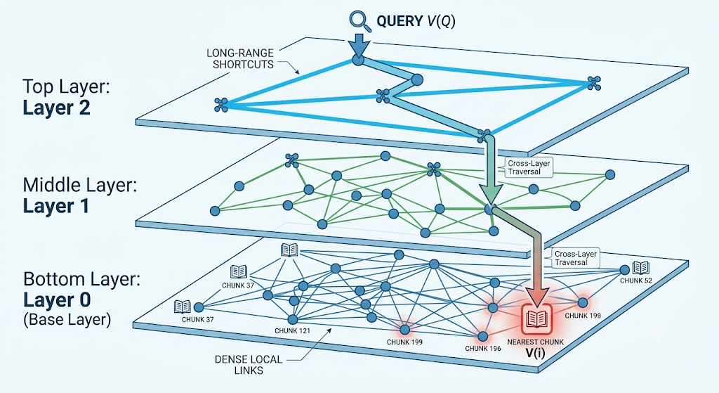
HNSW stands for Hierarchical Navigable Small World. The name sounds like a research paper that wants to scare beginners away. The idea is actually intuitive. Faiss’s HNSW structures maintain neighbor links between vectors, and the search structure uses entry points and linked neighbors across levels to navigate the space efficiently.
Think of it like a city with highways and side streets. If you want to reach a specific place, you do not walk randomly through every road in the city. You take major roads first, get close to the destination, and then move through smaller streets. HNSW does something similar. It starts from a high-level entry point, moves through the graph, and gradually reaches the best local matches.
This is why HNSW is popular in RAG systems. It tends to give strong recall and fast retrieval, which makes it attractive when quality matters. The trade-off is memory, because graph links take space. That is the engineering reality: better navigation usually means more structure to store.
🔴 IVF: The Shelf System
IVF stands for Inverted File Index. If HNSW is a city map, IVF is a library with organized shelves. Faiss describes IVF as an index where a quantizer assigns each vector to a list, and those lists act like posting lists or inverted lists. The point is to search only the most promising clusters instead of scanning the entire space.
That library metaphor is easy to remember. Imagine all your study PDFs are arranged by subject. Mathematics goes on one shelf. Physics on another. NLP on another. If a student asks about backpropagation, you do not search every shelf in the library. You go to the most relevant section first. IVF does that at the vector level.
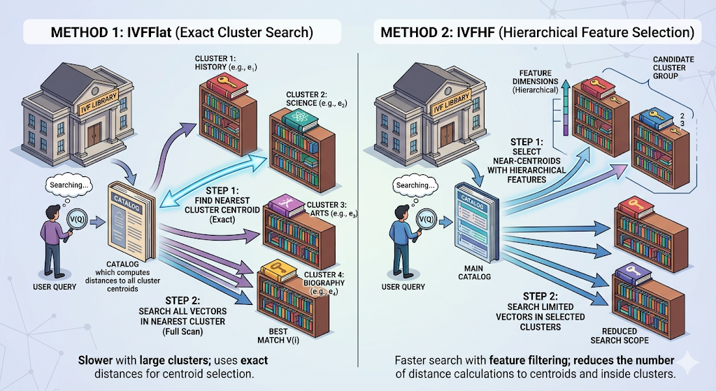
IVF is especially useful when the corpus becomes large and you want a search structure that clusters vectors before searching them. The trade-off is that a query may miss some neighbors near cluster boundaries, which is why ANN search is always about balance, not magic.
🔴 HNSW vs IVF
Beginners often ask which one is better. The honest answer is that both are useful, but they solve the problem in different ways. HNSW uses a navigable graph with multiple levels. IVF uses clustering and inverted lists. Faiss documents both as core retrieval structures, and that alone tells you they are not niche ideas. They are standard tools in large-scale vector search.
If you want a simple mental model, keep this in mind. HNSW feels like intelligent routing. IVF feels like smart grouping. HNSW often shines when you want very strong nearest-neighbor search behavior. IVF often shines when you want compact clusters and scalable search over a massive vector set. Neither is universally “best.” The right choice depends on your scale, latency needs, memory budget, and recall expectations.
🔴 Why Vector Search Is Still Not Enough
Now comes the part that surprises many beginners. Even after you have a strong vector search system, retrieval can still fail. Why? Because vector search is great at meaning, but not always great at exact words. If a user asks for “CS229 Assignment 4,” or “HR-2025 policy,” or “TensorFlow 2.18,” the exact tokens matter a lot. Semantic similarity alone may not always be enough. OpenSearch’s documentation makes this distinction clearly by contrasting BM25 keyword search with semantic search. This is where search becomes more mature.
Instead of choosing between meaning and keywords, production systems often combine both.
🔴 BM25 and Sparse Retrieval
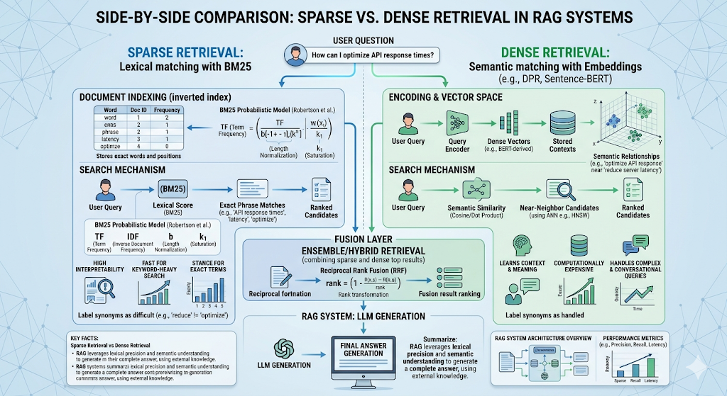
BM25 is one of the classic lexical ranking algorithms used in search engines. OpenSearch states that by default it uses Okapi BM25, which is a keyword-based algorithm that ranks documents based on term frequency and document length. In plain English, BM25 is very good when the user’s words matter exactly as written.
That makes BM25 the perfect counterpart to embeddings. Dense retrieval understands semantic meaning. BM25 understands literal words. When a student searches for a precise chapter number, formula name, policy code, or assignment title, BM25 can save the day. OpenSearch also explicitly notes that BM25 works well for keyword queries while semantic search is better when natural language understanding is needed.
🔴 Dense Retrieval
Dense retrieval is the embedding-based side of the house. Instead of comparing exact terms, it compares vector representations of meaning. That is the reason RAG became such a powerful pattern in the first place. It lets a system find passages that are relevant even if the wording is different. LangChain’s retrieval and knowledge-base guides describe this standard stack as documents, text splitters, embeddings, vector stores, and retrievers.
Dense retrieval is especially helpful when the user asks conceptually. “Explain gradient descent in simple words” is a meaning question. “What does section 4.2 say exactly?” is more of a lexical question. Real systems need both.
🔴 Hybrid Search
This is where hybrid search enters. Hybrid search combines sparse retrieval and dense retrieval so the system can capture both exact terms and semantic meaning. OpenSearch and Elasticsearch both document hybrid search patterns that blend keyword and vector search, and Elasticsearch specifically recommends Reciprocal Rank Fusion as a practical way to merge multiple result sets.
In the study assistant story, hybrid search is the moment the system stops being fragile. A question like “Explain Adam Optimizer from Page 7” benefits from meaning-based retrieval because of “Adam Optimizer,” but it also benefits from keyword search because “Page 7” is an exact reference. Hybrid search lets both signals help.
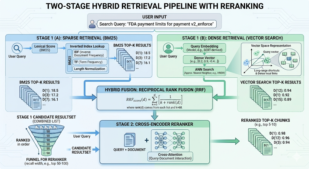
🔴 Reciprocal Rank Fusion
Once you have two result lists, you need a way to combine them. RRF, or Reciprocal Rank Fusion, is one of the cleanest methods for that job. Elasticsearch defines it as a way to combine multiple ranked result sets into a single result set, and notes that it requires no tuning. That is one reason it is so attractive in hybrid search pipelines.
The logic is beautifully practical. If a chunk appears near the top of both the BM25 list and the vector list, it probably deserves attention. RRF rewards that consistency. It does not obsess over whether one scoring system uses the same scale as the other. It simply trusts rank agreement.
🔴 Re-Ranking: The Final Judge
Retrieval is not done after the first search. The first search is a funnel, not the finish line. It brings back a set of candidates quickly, but some of them will be irrelevant or only loosely related. That is why the next stage is re-ranking. Sentence Transformers says Cross-Encoders are commonly used as second-stage rerankers in a retrieve-and-rerank pipeline.
The idea is simple. A retriever may pull back twenty or fifty chunks. A reranker then reads the query and each candidate together and assigns a better relevance score. Sentence Transformers explains that Cross-Encoders take the query and the document simultaneously and output a single relevance score. That is why they are more accurate than plain embedding search for final ordering, even though they are slower.
That trade-off matters. Retrieval gets you speed. Re-ranking gets you precision. Real systems need both.
🔴 Metadata Filtering
Not every question should search every document. If the student asks about NLP, the system should not waste time searching chemistry notes. That is where metadata filtering becomes useful. LangChain’s retriever and vector store integrations show that metadata filters can be applied during search, and Qdrant in particular supports rich metadata filtering.
This sounds minor, but it is a real production boost. Metadata can restrict results by subject, file type, date, source, author, department, or access level. In an educational assistant, metadata filtering can keep the retrieval focused on the exact course or chapter the user cares about.
🔴 Query Expansion and Multi-Query Retrieval
Users are not always precise. They ask messy questions, vague questions, and sometimes the wrong question entirely. One way to help is to generate multiple related versions of the query. LangChain’s MultiQueryRetriever documentation describes this as creating multiple variants of a question with similar meaning to the original query. LangChain also notes that multiple searches may be allowed for a single user query in RAG workflows.
This is a powerful trick because one query may miss the right passage while another query hits it perfectly. A system that searches multiple variants is often more forgiving and more useful, especially on educational content where users ask in rough, incomplete language.
🔴 Why This Part Matters
Part 2 is where RAG stops being a simple demo and starts feeling like a real retrieval system.
We moved from “store vectors and search them” to the richer world of ANN search, graph navigation, cluster-based search, lexical search, hybrid retrieval, ranking fusion, reranking, and filtering.
Faiss, OpenSearch, Elasticsearch, Sentence Transformers, Qdrant, and LangChain all describe pieces of this stack in their own ways, but the deeper truth is simple: good RAG is good retrieval, and good retrieval is a layered system, not a single trick.
🔴 What Comes Next
In the next article, I will cover the part most people skip until they need it badly: what happens when retrieval itself is not enough. That means Agentic RAG, CRAG, Self-RAG, GraphRAG, evaluation, correction, and the systems that decide when to search again instead of answering too early.
LangChain’s agentic RAG guidance already points in that direction, where the model can decide when to use a retriever tool, and Graph-based retrieval is also emerging as a structured extension of vector search.
🔴 Complete RAG Roadmap
Part 1: RAG Explained From Scratch: How PDFs Become Searchable Knowledge for AI
Part 2: How RAG Actually Finds Answers: HNSW, IVF, BM25, Hybrid Search and Re-Ranking
Next Article Part 3: Beyond Basic RAG: Agentic RAG, CRAG, Self-RAG and GraphRAG Explained
Mehul Ligade
X: @MehulLigade
LinkedIn: linkedin.com/in/mehulcode12
How RAG Actually Finds Answers (Part 2): HNSW, IVF, BM25, Hybrid Search and Re-Ranking | M011 |… was originally published in Towards AI on Medium, where people are continuing the conversation by highlighting and responding to this story.