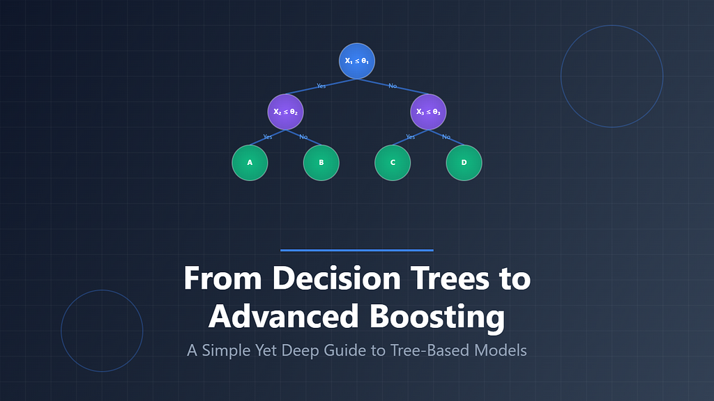
From Decision Trees to Advanced Boosting: A Simple Yet Deep Guide to Tree-Based Models

digitado ⋅ 7 de May de 2026

If you’ve worked with tabular data, you’ve likely noticed something:

No matter how advanced deep learning becomes, tree-based models often outperform everything else.

From credit risk prediction to medical decision support, models like XGBoost, LightGBM, and CatBoost dominate real-world machine learning tasks.

But why are they so powerful?
And how did we get from a simple decision tree to these highly optimized algorithms?

This article breaks it down from first principles — in a way that builds intuition before diving into advanced concepts.

Imagine you’re trying to decide whether a patient is at risk based on some features:

Age
Blood pressure
Cholesterol

A human might think like this:

“If age is high and cholesterol is high → risk is high.”

That’s exactly how a Decision Tree works.

1. Decision Trees — Learning Like a Human

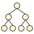
A Decision Tree is essentially a series of yes/no questions.

Example:

Is age > 50?
Yes → Go right
No → Go left
Is cholesterol high?
Yes → High risk
No → Low risk

It keeps splitting the data until it reaches a final decision.

How Decision Trees Decide Splits: Gini Index and Entropy

When a decision tree is built, its most important task is deciding how to split the data at each step.

At every node, the model asks a simple question:

“Which feature split will separate the classes in the best possible way?”

To answer this, the tree needs a way to measure how “mixed” or “pure” a group of data is. This is where Gini Index and Entropy come in.

Both are impurity measures, meaning they tell us how disorganized a dataset is at a given node.

Gini Index — Measuring Impurity

The Gini Index tells us how often a randomly chosen data point would be incorrectly classified if it were labeled according to the class distribution in a node.

In simpler terms:

If a node contains only one class, it is perfectly pure.
If it contains many classes mixed together, it is impure.

Formula

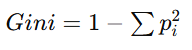
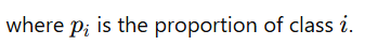
Intuition

If all samples belong to one class, Gini = 0
If classes are evenly mixed, Gini increases

The higher the Gini value, the more mixed the node is.

Example

If a node contains only one class (for example, all dogs):

This means the node is completely pure.

If a node contains 50% dogs and 50% cats:

This represents a mixed and impure node.

Key Idea

Decision trees try to choose splits that reduce the Gini Index as much as possible, because lower impurity means better separation of classes.

Entropy — Measuring Uncertainty

Entropy comes from information theory and measures the level of uncertainty in a dataset.

While Gini focuses on impurity, entropy focuses on:

“How uncertain are we about the class of a data point?”

If a node is perfectly pure, there is no uncertainty.
If classes are evenly mixed, uncertainty is at its highest.

Formula

Intuition

Low entropy means the model is confident
High entropy means the model is uncertain

Example

For a pure node (all samples belong to one class):

Entropy=0

There is no uncertainty.

For a balanced node (50% two classes):

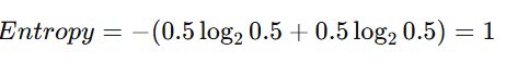
This is maximum uncertainty.

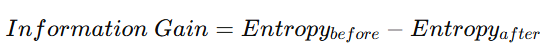
Information Gain

Decision trees using entropy aim to maximize information gain, which measures how much uncertainty is reduced after a split.

Gini vs Entropy — What’s the Difference?

Both Gini Index and Entropy measure impurity, but they do it in slightly different ways.

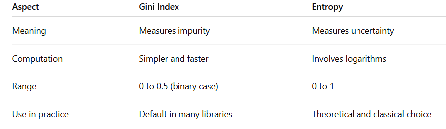
In most modern implementations, including scikit-learn, Gini Index is often preferred because it is computationally efficient and produces very similar results to entropy.

Final Intuition

Think of it this way:

A decision tree is constantly asking:

“Which split makes the data most organized?”

Gini Index measures how messy the data is
Entropy measures how uncertain the prediction is

Both guide the tree toward cleaner and more separable groups of data.

Ensemble Learning: How Weak Models Become Powerful Predictors

Single machine learning models often struggle with one of two problems:

They are too simple and underfit the data
Or they are too complex and overfit the data

Ensemble learning solves this by combining multiple models to create a stronger one.

The core idea is simple:

“Many weak models together can create a strong model.”

There are three main ensemble strategies:

Bagging
Boosting
Stacking (brief mention)

We will focus on bagging and boosting, since they form the foundation of modern tree-based systems like XGBoost, LightGBM, and CatBoost.

1. Bagging — Building Independent Models

Bagging stands for Bootstrap Aggregation.

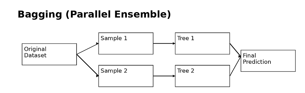
How It Works

Take the original dataset
Create multiple random samples (with replacement)
Train a model on each sample independently
Combine their outputs (majority vote or average)

Intuition

Think of asking multiple doctors the same question:

Each doctor sees slightly different patient data
Each gives an independent opinion
Final decision = majority vote

No doctor learns from another.

Why Bagging Works

Bagging reduces variance.

Individual decision trees are unstable
Small data changes → very different trees
Averaging them stabilizes predictions

Python Example (Bagging with Decision Trees)

from sklearn.ensemble import BaggingClassifier
from sklearn.tree import DecisionTreeClassifier
from sklearn.datasets import load_breast_cancer
from sklearn.model_selection import train_test_split
from sklearn.metrics import accuracy_score

X, y = load_breast_cancer(return_X_y=True)
X_train, X_test, y_train, y_test = train_test_split(X, y)

base_model = DecisionTreeClassifier()

model = BaggingClassifier(
    estimator=base_model,
    n_estimators=50,
    random_state=42
)

model.fit(X_train, y_train)
y_pred = model.predict(X_test)

print("Accuracy:", accuracy_score(y_test, y_pred))

2. Boosting — Learning from Mistakes

Boosting is fundamentally different.

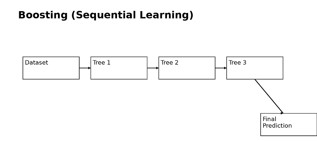
Instead of training models independently, boosting trains models sequentially.

Each new model focuses on correcting the mistakes of the previous ones.

How It Works

Train a weak model
Identify errors
Train next model to fix those errors
Repeat
Combine all models (weighted sum)

Intuition

Think of a student improving over time:

First attempt → many mistakes
Teacher highlights errors
Student improves step by step

Each new model is smarter than the previous one.

Why Boosting Works

Boosting reduces bias + variance.

Learns complex patterns
Focuses on hard samples
Improves performance iteratively

Python Example (Basic Gradient Boosting)

from sklearn.ensemble import GradientBoostingClassifier

model = GradientBoostingClassifier(
    n_estimators=100,
    learning_rate=0.1,
    max_depth=3
)

model.fit(X_train, y_train)
y_pred = model.predict(X_test)

print("Accuracy:", accuracy_score(y_test, y_pred))

3. XGBoost — Optimized Gradient Boosting

XGBoost is one of the most widely used ML algorithms in the world.

What Makes It Special?

1. Regularization

It penalizes complex trees:

Prevents overfitting
Encourages simpler models

2. Second-Order Optimization

Instead of only using errors, it uses:

Gradient (first derivative)
Hessian (second derivative)

This improves accuracy and convergence.

3. Handles Missing Values Automatically

Learns best direction for missing splits.

Python Example

from xgboost import XGBClassifier

model = XGBClassifier(
    n_estimators=200,
    learning_rate=0.05,
    max_depth=6,
    subsample=0.8,
    colsample_bytree=0.8
)

model.fit(X_train, y_train)
y_pred = model.predict(X_test)

print("Accuracy:", accuracy_score(y_test, y_pred))

4. LightGBM — Speed and Scalability

LightGBM is designed for large-scale data.

Key Idea: Histogram-Based Learning

Instead of using raw values:

Continuous features are grouped into bins
Splits are computed on bins

This makes it extremely fast

Tree Growth Difference

XGBoost → level-wise growth
LightGBM → leaf-wise growth

Leaf-wise growth:

Focuses on most important leaf
Leads to better accuracy
But can overfit if not controlled

Python Example

from lightgbm import LGBMClassifier

model = LGBMClassifier(
    n_estimators=200,
    learning_rate=0.05,
    num_leaves=31
)

model.fit(X_train, y_train)
y_pred = model.predict(X_test)

print("Accuracy:", accuracy_score(y_test, y_pred))

5. CatBoost — Best for Categorical Data

CatBoost is designed to handle categorical features directly.

The Problem

Traditional models require encoding:

One-hot encoding → too large
Label encoding → misleading

CatBoost Solution

Uses ordered target encoding:

Converts categories into meaningful statistics
Avoids data leakage
Uses only past information during encoding

Key Feature: Symmetric Trees

Same structure at each level
Faster inference
More stable training

Python Example

from catboost import CatBoostClassifier

model = CatBoostClassifier(
    iterations=200,
    depth=6,
    learning_rate=0.05,
    verbose=0
)

model.fit(X_train, y_train)
y_pred = model.predict(X_test)

print("Accuracy:", accuracy_score(y_test, y_pred))

6. Final Comparison

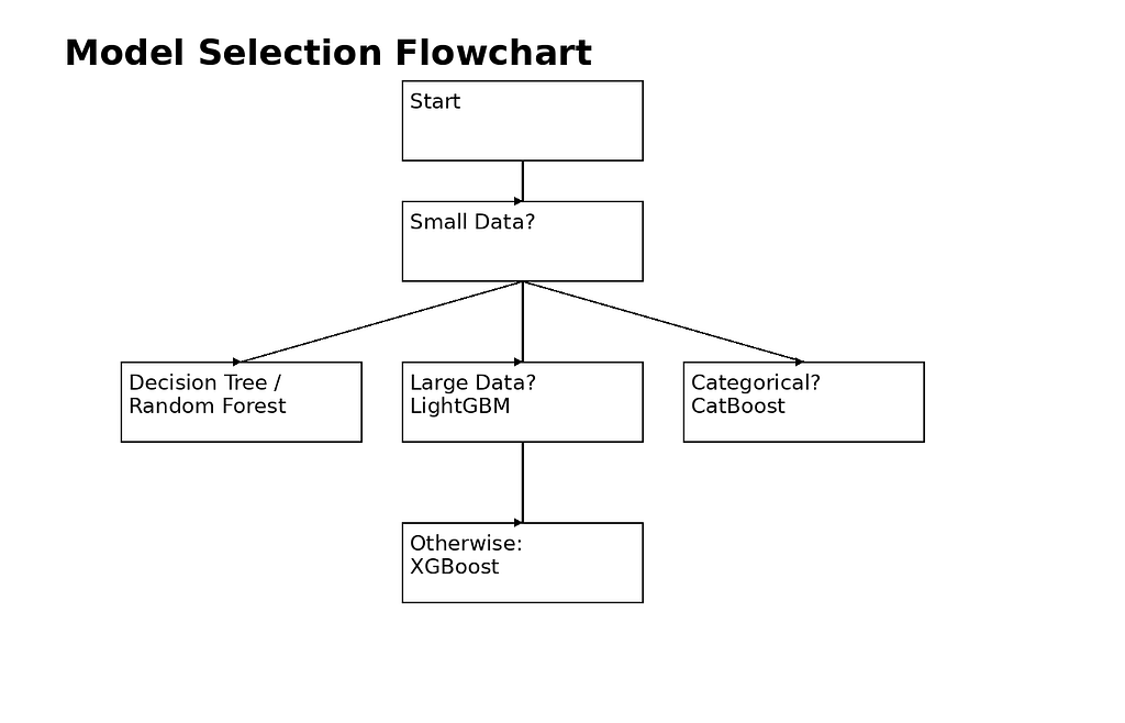
7. Selection of Model

Final Intuition

Bagging = “many independent opinions”
Boosting = “learning from mistakes step-by-step”
XGBoost = “optimized disciplined boosting”
LightGBM = “fast and aggressive boosting”
CatBoost = “smart handling of categorical data”

References

scikit-learn — Machine Learning in Python
XGBoost — Official Documentation
LightGBM — Official Documentation
CatBoost — Official Documentation
Breiman, L. (2001). Random Forests
Chen, T., & Guestrin, C. (2016). XGBoost: A Scalable Tree Boosting System
Ke, G. et al. (2017). LightGBM: A Highly Efficient Gradient Boosting Decision Tree
Prokhorenkova, L. et al. (2018). CatBoost: Unbiased Boosting with Categorical Features

From Decision Trees to Advanced Boosting: A Simple Yet Deep Guide to Tree-Based Models was originally published in Towards AI on Medium, where people are continuing the conversation by highlighting and responding to this story.

Like 0

Liked Liked