Modern biology has a data problem, but not the kind you might expect. Generating massive datasets from wet-lab experiments has become routine thanks to falling sequencing costs and standardized protocols. The bottleneck is what comes after: processing, analyzing, and interpreting that data. A single spatial transcriptomics run (maps gene expression across physical tissue space) can produce hundreds of thousands of cell-level observations across hundreds of genes. The analytical pipeline to go from raw counts to biological insight involves a long chain of preprocessing, dimensionality reduction, and cell type annotation, each step with its own tooling and failure modes. It’s a gap that separates the bench scientist from the biological insight, and it’s exactly the problem that LatchBio is building to solve.

This past fall, a team from Machine Learning at Berkeley partnered with LatchBio, a San Francisco-based biotech infrastructure company whose founding team includes ML@B alumni, to stress-test and evaluate the agentic capabilities of their data analysis platform. Over ten weeks, our team worked hands-on with the first version of LatchBio’s console agent, probing its ability to handle real spatial transcriptomics workflows and developing a structured evaluation framework for systematically measuring its performance.

It’s worth noting upfront that the agent has improved substantially since our engagement, the capabilities and limitations described here reflect the v1 system we benchmarked, not the current state of the product.

What LatchBio Is Building

LatchBio provides an integrated platform that bridges the gap between bioinformatics tooling and the scientists who need to use it. Their platform supports data from over 40 kits and instruments and is designed for everyone from bench scientists who may have limited computational experience to R&D leadership making decisions based on analytical outputs. They’ve raised roughly $32.8M from investors including Lux Capital, General Catalyst, and Caffeinated Capital.

At the center of their current work is an agentic console built around Latch Plots, a Jupyter notebook-like framework that automates the most labor-intensive parts of bioinformatics data curation. The user can prompt the agent to complete discrete tasks, such as data ingestion, count matrix construction, quality control, transformation, cell typing, and metadata harmonization. Once prompted, the LLMs operate in sandboxed environments, write and validate their own code, and produce reports with chain-of-thought reasoning. The human scientist (user) reviews and approves the output at each stage before the pipeline advances.

Sitting With the Data

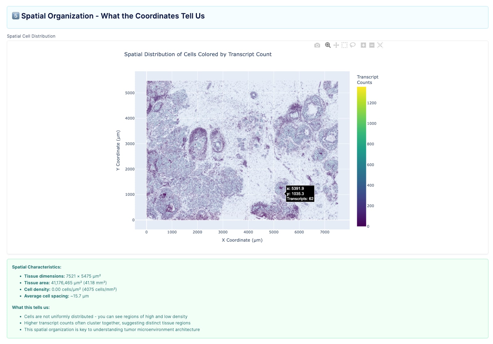
Before we could evaluate the agent, we needed to understand the data ourselves. Most of what we worked with came from 10x Genomics spatial transcriptomics datasets, primarily Xenium FFPE (formalin-fixed paraffin-embedded) human breast cancer samples, with some Visium data mixed into the same directories. Xenium is an in situ transcriptomics platform that provides subcellular-resolution gene expression measurements across a targeted panel of several hundred genes, while Visium captures whole-transcriptome data at spot-level resolution. Both are spatially resolved, but they differ significantly in gene panel size, resolution, file structure, and the analytical approaches appropriate for each.

We spent considerable time reading through the associated literature, particularly the 10x Genomics paper “High resolution mapping of the tumor microenvironment using integrated single-cell, spatial and in situ analysis”, to ground ourselves in what correct analysis looked like for these datasets. We wanted to approach the agent from the perspective of a genomicist who knows what good results should look like, rather than simply asking the agent to reproduce known figures.

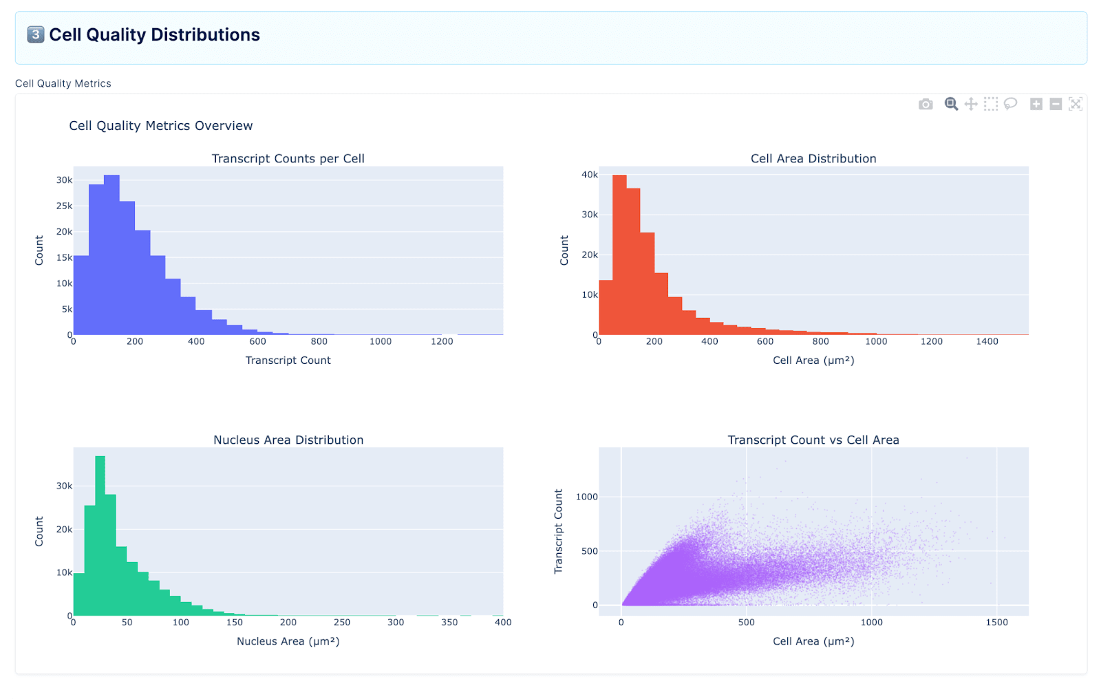
A typical Xenium breast cancer dataset might contain on the order of 167,000 cells across a panel of ~541 genes. The standard analytical workflow in a tool like Scanpy involves QC filtering (removing cells with too few detected genes or too few total counts), library-size normalization, log transformation, PCA for dimensionality reduction, neighborhood graph construction, Leiden clustering, and UMAP embedding for visualization. Downstream, you’d run differential expression to find marker genes per cluster and attempt cell type annotation based on known marker panels. Each of these steps has parameters that meaningfully affect results — clustering resolution, neighbor count, the choice of DE test — and getting them wrong can produce clusters that are artifacts of preprocessing rather than reflections of real biology.

Working With the Agent to Reproduce Ground Truth

Rather than jumping straight to formal benchmarks, we approached the agent conversationally. We uploaded raw files through LatchBio’s console, prompted it to load data and generate plots, and observed what it produced. The console’s interface made this straightforward: you navigate to the Plots section, attach specific data files (in our case, the Xenium FFPE Human Breast Cancer Rep 1 outputs), and provide a natural language prompt. The agent then executes a full analysis pipeline, returning summaries, visualizations, and a step-by-step account of its reasoning.

What emerged was a much more iterative process than we anticipated. We’d prompt the agent, see something that wasn’t quite right, and nudge it in a different direction. Early on, we found that the agent could successfully run unsupervised clustering (Leiden + UMAP) and produce groupings that reflected real biological structure, such as separating broad compartments like tumor, stroma, and immune populations. But it struggled with the next step: taking those clusters and annotating them with specific cell type labels based on marker gene expression. A lot of the initial work was simply mapping the boundaries of what the agent could and couldn’t do on real data, where it broke, where it hallucinated, and where it surprised us.

One task that made this particularly clear was identifying Visium outputs inside a shared 10x dataset that also contained Xenium files. On paper, this sounds straightforward, but in practice it requires the agent to pick up on file structure conventions and modality-specific details that are usually implicit to someone familiar with the ecosystem. Things like the presence of spatial/ directories, barcode formats, and the distinction between spot-level and cell-level count matrices.

To even define the task properly, we had to read through the paper ourselves, understand the intended analysis, and guide the agent from an incorrect answer to a correct one. That corrected output then effectively became our ground truth.

This back-and-forth shaped our philosophy for the rest of the project. Rather than prescribing what the agent should do upfront, we let it run, observed where it failed, and used those failures to define evaluation criteria. Ground truth emerged from the process of iterating with the agent, not from a pre-existing rubric.

Building the Eval Framework

Once we had a sense of the agent’s capabilities and failure modes, we moved to structured evaluation. We converged on a JSON-based eval format with four core components: a prompt (the task instruction), a dataset reference (a Latch URI pointing to the raw data), a ground truth (the expected output), and an evaluation metric (a scoring function and pass threshold).

We used the agent itself to help generate evals. After the agent demonstrated comfort with a dataset through exploratory analysis, we prompted it to identify tasks suitable for AI evaluation, then asked it to produce eval to evaluate its own performance. We provided an example from LatchBio’s prior evals to the agent, and it was able to produce well-formed evals that were usable without significant manual editing.

It’s worth noting that this self-generation approach is meant for probing the boundaries of a single system’s capabilities (where it works and where it breaks down), but has obvious limitations for cross-framework benchmarking, since the agent naturally generates tasks within its own competence distribution.

We then fed those evals back to the agent in a fresh console session (attaching the same data files and providing the eval tasks as prompts) and observed how it performed on its own generated benchmarks. This self-evaluation loop was informative: it helped us identify whether the agent’s eval generation was producing tasks that were too easy (the agent always passes), too hard (the agent fails for mechanical reasons like file parsing errors or malformed output rather than analytical shortcomings), or well-calibrated.

We withheld not just the ground truth but also the grading metric and pass threshold during the agent’s initial attempt to solve the eval. The agent received the task instruction and data, but had no knowledge of how its output would be scored or what specifically constituted a passing result. Only after it produced an output did we reveal the full eval JSON and review its work against the rubric. This made it easy to separate two distinct failure modes: pipeline-execution failures, where the agent couldn’t complete the analysis at all, and rubric-matching failures, where the agent completed a reasonable analysis but its output didn’t align with our specific scoring criteria.

A Concrete Example: Luminal Marker Identification

One eval we developed in detail was derived from the 10x breast cancer paper. The task was: given raw Xenium data, find the genes that best distinguish cancer cells from everything else in the tissue.

Concretely, the agent was given a single compound instruction — load the data in Scanpy, run one-vs-all differential expression using t-test_overestim_var (logFC > 0, adjusted p-value ≤ 0.05, use_raw=False), rank genes by logFC then −log₁₀(adjusted p), convert to uppercase gene symbols, and identify clusters expressing canonical luminal cancer cell markers (KRT8, KRT18, KRT19, EPCAM).

The grading used a label-set Jaccard index: we compared the agent’s top-k predicted marker genes against the ground truth marker set, with a pass threshold of Jaccard ≥ 0.36 using the top 8 agent markers. We chose Jaccard because it naturally handles partial overlap and penalizes both missing true markers and including irrelevant ones, without being as brittle as exact-match scoring.

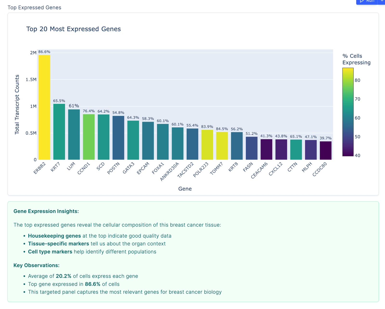
The agent’s output was substantive. It processed 167,780 cells across 541 genes, applied QC filtering, ran the full Leiden clustering pipeline (resolution 0.5, 9 clusters), and identified 4 clusters that appeared to correspond to luminal cells (epithelial cells that line breast ducts and are the cell of origin for some subtypes of breast cancer). The agent made this identification by looking for clusters with high expression of KRT8 and EPCAM, two well-established luminal markers. Notably, two other canonical markers — KRT18 and KRT19 — were absent from the Xenium gene panel entirely, and the agent correctly flagged this rather than hallucinating results for genes that weren’t measured. It adapted its strategy accordingly, which is the kind of context-aware behavior that distinguishes genuine analysis from pattern-matching. Across those 4 luminal clusters, the agent returned 236 unique marker genes.

The analysis revealed real biological heterogeneity within the luminal compartment: a classical luminal cluster with hormone receptor expression (ESR1, PGR, GATA3, FOXA1), an adhesion-enriched cluster (CEACAM6, TACSTD2), a basal-luminal hybrid population co-expressing KRT5/KRT14 with luminal markers, and a small cluster with matrix remodeling signatures. These findings aligned well with the published literature and gave us confidence that the agent was performing genuine analysis rather than pattern-matching on superficial cues.

Common failure modes we cataloged across multiple evals included universal markers (like housekeeping genes) dominating top-ranked lists, subset-specific markers being diluted when aggregated across multiple clusters, and contamination from fibroblast or stromal gene programs appearing in predicted epithelial marker sets.

Reflections and What’s Next

Over time, our approach to working with the agent naturally shifted toward smaller, quiz-style tasks (file identification, clustering parameter selection, basic cell typing) scored with simple metrics. This wasn’t a second formal evaluation framework; it was how we learned to probe the agent most effectively during day-to-day interaction. Compared to the compound instructions in our structured evals, these smaller tasks gave us faster, clearer signals on what the agent understood versus what it was guessing at.

The agent’s core strength is clear: its ability to consume complex, high-dimensional biological data and produce coherent, end-to-end analysis is genuinely useful. Tasks that would normally require a scientist to wrangle Scanpy, NumPy, and Pandas can be handled conversationally. For researchers without deep computational backgrounds, this is a meaningful reduction in the barrier between data and insight.

One area where we see room for improvement is transparency during execution. The agent’s analysis can take several minutes, and during that time the process is largely opaque from the console. Showing intermediate reasoning steps, partial results, or even just which stage of the pipeline the agent is currently executing would better align with how scientists think about trusting computational outputs.

We also found that the agent’s performance was meaningfully sensitive to prompt framing. Broad, open-ended instructions sometimes led to overly ambitious subtask decomposition, while more targeted prompts produced more reliable results. This suggests that continued investment in domain-specific prompt engineering, and potentially more structured task decomposition within the agent itself, will yield significant returns.