The Hidden Cost of Large Weights: Understanding Regularization in Machine Learning

digitado ⋅ 23 de June de 2026

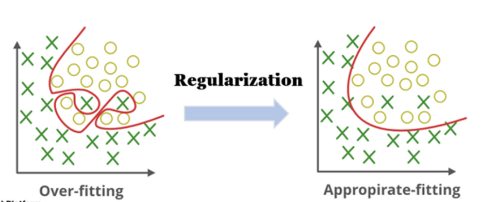
One of the first things I learned in Machine Learning was that reducing loss is important. After all, a lower loss usually means better predictions. So naturally, I assumed that if a model keeps reducing the training loss, it must be getting better. But that assumption isn’t always true. Sometimes a model becomes so good at fitting the training data that it starts memorizing it instead of learning meaningful patterns. As a result, it performs extremely well on the data it has already seen but struggles when presented with new examples. This phenomenon is known as Overfitting.

A useful way to think about overfitting is that the model becomes overly specialized. Instead of learning the underlying relationship in the data, it begins learning the noise, random fluctuations, and peculiarities of the training set. The result is a model that looks impressive during training but fails to generalize well in the real world. An overfitted model, however, might start learning accidental patterns that only exist in the training dataset. It may treat random variations as important signals and become unnecessarily complex.

This raises an important question:

If increasing model complexity can lead to overfitting, how do we prevent a model from becoming too complex in the first place?

One of the most effective solutions is Regularization. Rather than allowing the model to use any weights it wants, Regularization introduces a penalty for excessively large weights and encourages the model to learn simpler, more generalizable solutions. And surprisingly, that small change can have a huge impact on performance.

What Is Regularization?

At its core, Regularization is a technique used to reduce overfitting by discouraging the model from learning excessively large weights. Normally, during training, a machine learning model tries to minimize a loss function. The loss measures how far the model’s predictions are from the actual values. The lower the loss, the better the model appears to be performing. Without regularization, the optimization process only cares about reducing this prediction error. As a result, the model is free to use any weights necessary to achieve a lower loss, even if those weights become extremely large.

This is where Regularization changes the game. Instead of minimizing only the original loss, we modify the objective function by adding an additional penalty term. The penalty increases whenever the model starts assigning very large values to its weights.

In other words, the model now has two goals:

Fit the training data well.
Keep the weights reasonably small.

This creates a tradeoff between accuracy and complexity.

The Most Important Intuition

When I first learned Regularization, I assumed it somehow helped reduce the loss directly. But that’s not actually what happens. Regularization does not directly improve predictions. Instead, it changes what the optimization algorithm considers to be a “good” solution. A model with slightly higher prediction error but smaller weights may now be preferred over a model with extremely large weights. You can think of it like this: Imagine two students taking an exam.

Student A gets 95 marks but uses ten pages of rough work.

Student B gets 93 marks using only two pages.

If we introduce a penalty for excessive rough work, Student B may become the preferred solution. Regularization applies a similar idea to machine learning models. Large weights become expensive. As a result, Gradient Descent naturally starts preferring simpler solutions.

Why Does This Help?

Large weights often indicate that the model is becoming too dependent on specific features. Instead of learning general patterns, it may start amplifying tiny fluctuations in the training data. This makes the model more sensitive to noise and increases the risk of overfitting. By discouraging large weights, Regularization encourages the model to focus on patterns that consistently appear across the dataset. The result is often a model that performs slightly worse on the training data but significantly better on unseen data. And in machine learning, that’s usually a tradeoff worth making.

But how exactly does the penalty influence the learning process?

To answer that, we need to look at the modified cost function and understand the role of a very important parameter: λ (lambda), which controls the strength of regularization.

Understanding the Role of λ (Lambda)

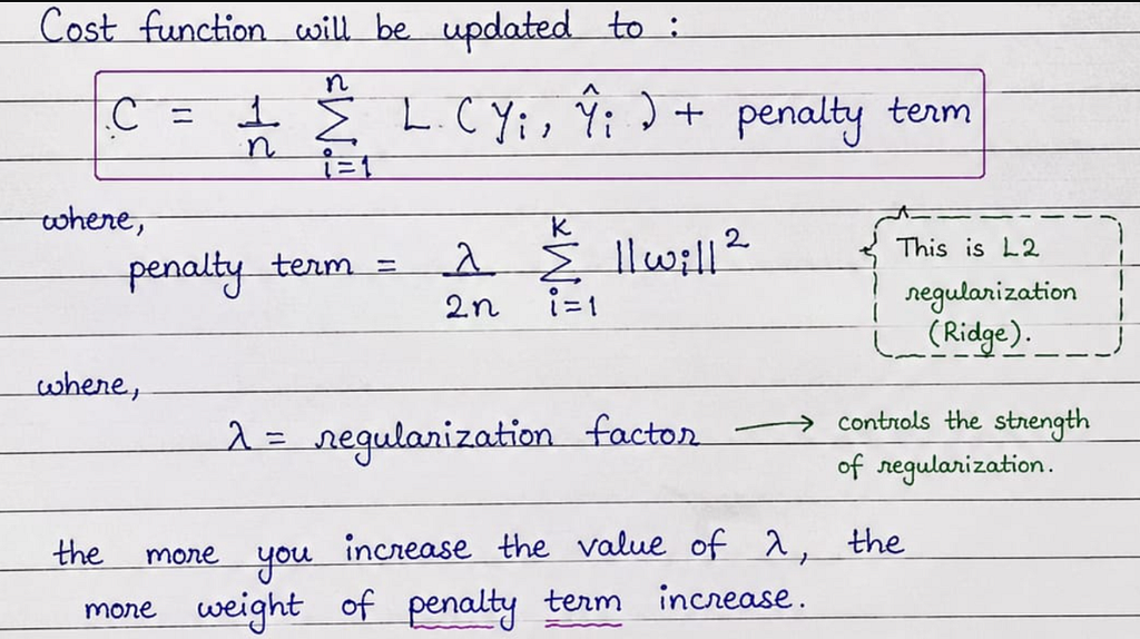
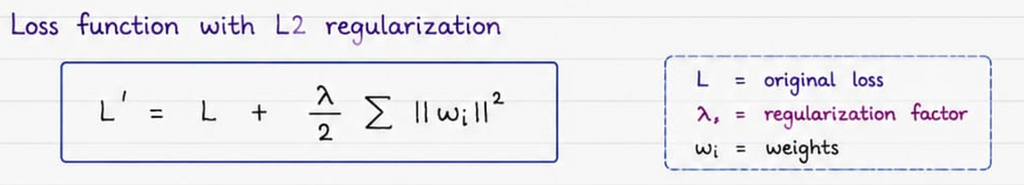
Once regularization is added, the cost function becomes:

Cost = Original Loss + PenaltyCost

For L2 Regularization, the penalty term is:

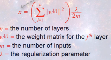
At first glance, λ (lambda) may look like just another parameter. But in reality, it controls one of the most important tradeoffs in machine learning. Think of λ as a knob that controls how strongly we penalize large weights. As λ increases:

The penalty becomes more important.
Large weights become more expensive.
The model is forced to stay simpler.

As λ decreases:

The penalty becomes weaker.
The model gets more freedom.
Large weights are less restricted.

The Balancing Scale Analogy

One way to visualize λ is as a balancing scale. On one side, we have: Data Fitting, how well the model explains the training data. On the other side, we have: Model Simplicity, how small and controlled the weights remain. Regularization tries to balance these two objectives. The value of λ determines which side receives more importance.

What Happens When λ Is Too Small?

When λ is close to zero, the penalty term becomes almost insignificant. The optimization process behaves nearly the same as ordinary training. The model focuses almost entirely on reducing prediction error. This often leads to:

Very large weights
Complex decision boundaries
Increased risk of overfitting

The model may perform extremely well on training data but struggle on unseen examples.

What Happens When λ Is Too Large?

Now imagine increasing λ significantly. The penalty term begins dominating the objective function. The model becomes heavily restricted and starts avoiding large weights at all costs. As a result:

Weights become very small.
The model becomes overly simple.
Important patterns may be ignored.

This can lead to Underfitting. Instead of memorizing the training data, the model now struggles to learn enough from it.

Finding the Sweet Spot

The goal is not to maximize or minimize λ. The goal is to find a balance. A good λ value allows the model to: Learn meaningful patterns, avoid overly large weights, generalize well to unseen data This is why λ is usually treated as a hyperparameter and tuned experimentally.

How Regularization Actually Works: The Idea of Weight Decay

So far, we’ve seen that regularization adds a penalty term to the loss function. But an important question still remains: How does this penalty actually affect the weights during training?

To answer this, we need to look at the weight update equation used in Gradient Descent. Without regularization, the update rule is:

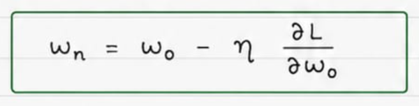
This update rule simply moves the weights in the direction that reduces the prediction error.

What Changes With L2 Regularization?

When L2 Regularization is introduced, the loss function becomes:

Now the gradient must account for both terms.

After differentiation, the update rule becomes:

At first glance, this equation may look intimidating. But the most important part is: (1−ηλ/n)

The Hidden Shrinking Effect

Notice something interesting. The term (1−ηλ/n) is usually slightly smaller than 1. That means every update multiplies the weight by a value less than 1. As training continues:

10 → 9.8 → 9.6 → 9.4 ...

The weights gradually shrink. This phenomenon is called: Weight Decay The weights are literally decaying over time.

Why Is This Useful?

Large weights often indicate that the model is relying heavily on specific features. This makes the model more sensitive to noise and increases the risk of overfitting. Weight Decay continuously pushes weights toward smaller values. As a result:

The model becomes simpler.
Individual features become less dominant.
Generalization usually improves.

Instead of allowing a few weights to become extremely large, the learning process naturally keeps them under control.

L2 Regularization works because it introduces a small shrinking force during every gradient update. Instead of only chasing lower loss, the model is constantly encouraged to keep its weights under control. This simple mechanism is the reason L2 Regularization is often called: weight decay.

L1 vs L2: Similar Goal, Different Behavior

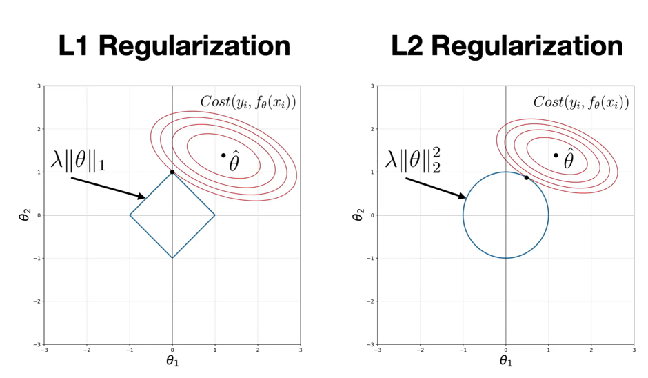
Up to this point, we’ve discussed L2 Regularization and how it gradually shrinks weights through Weight Decay. However, L2 is not the only regularization technique available. Another widely used approach is L1 Regularization, commonly known as Lasso Regression. At first glance, both techniques seem very similar. Both:

Add a penalty term to the loss function.
Discourage large weights.
Help reduce overfitting.
Improve generalization.

But there is one major difference: L2 shrinks weights. L1 can eliminate them entirely. And that difference changes everything.

L2 Regularization (Ridge)

L2 Regularization adds the following penalty:

λ∑W²

Notice that the weights are squared. Because larger weights produce much larger penalties, the optimization process continuously pushes them toward smaller values. However, something interesting happens: The weights usually become very small, but they rarely become exactly zero. For example:

Before:
[8.2, 5.1, 2.8, 0.9]

After L2:
[4.1, 2.3, 1.2, 0.3]

All features remain in the model. They simply contribute less. You can think of L2 as: “Keep all features, but don’t let any of them dominate.”

L1 Regularization (Lasso)

L1 Regularization uses a different penalty:

λ∑∣W∣

Instead of squaring the weights, it uses their absolute values. This small mathematical change leads to very different behavior. For example:

Before:
[8.2, 5.1, 2.8, 0.9]

After L1:
[4.5, 1.8, 0, 0]

Some weights become exactly zero. When a weight becomes zero, the corresponding feature effectively disappears from the model. This property is known as: Sparsity. A sparse model contains many zero-valued coefficients.

Why Is Sparsity Useful?

Imagine a dataset with 100 features. Not all of them are equally important. Some features genuinely help make predictions. Others contribute very little. L1 Regularization automatically removes many of those less useful features by pushing their weights to zero. As a result: Simpler models, Reduced complexity, Built-in feature selection. This is one of the reasons Lasso is often used when interpretability is important.

Regularization in Practice

Theory is important, but I wanted to see how regularization actually affects a model in practice. To explore this, I trained two neural networks on the same dataset:

Model 1: Without Regularization
Model 2: With L1 Regularization

The architecture remained identical. The only difference was the addition of a regularization term.

Without Regularization

model1 = Sequential()

model1.add(Dense(128, input_dim=2, activation="relu"))
model1.add(Dense(128, activation="relu"))
model1.add(Dense(1, activation="sigmoid"))

With L1 Regularization

model2 = Sequential()

model2.add(
    Dense(
        128,
        input_dim=2,
        activation="relu",
        kernel_regularizer=tf.keras.regularizers.l1(0.001)
    )
)

model2.add(
    Dense(
        128,
        activation="relu",
        kernel_regularizer=tf.keras.regularizers.l1(0.001)
    )
)

model2.add(Dense(1, activation="sigmoid"))

Notice that the only change is:

kernel_regularizer=tf.keras.regularizers.l1(0.001)

This adds an L1 penalty to the loss function and encourages the model to keep weights small.

Observing the Results

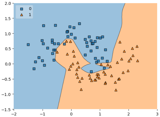
The model without regularization learns a more flexible decision boundary. While it captures the training data well, it is also more likely to fit noise and become overly complex.

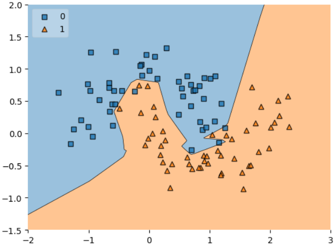
After introducing L1 Regularization, the decision boundary becomes smoother and less sensitive to small fluctuations in the data. The model is encouraged to learn simpler patterns that generalize better.

Looking at the Weights

To verify the effect of L1 Regularization, I compared the distribution of weights learned by both models.

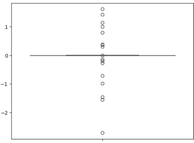
The regularized model contains many more weights close to zero. This is exactly what we expect from Lasso Regularization. Instead of allowing every feature to contribute equally, the model gradually removes weak contributors by pushing their weights toward zero. As a result:

Model complexity decreases.
Unimportant features lose influence.
Generalization often improves.

Key Observation

One of the most interesting observations was that Regularization doesn’t improve performance by learning new information. Instead, it improves performance by preventing the model from becoming unnecessarily complex. In other words: Regularization doesn’t make the model smarter; it helps the model stay disciplined.

Conclusion

Regularization is one of the most effective techniques for controlling overfitting in machine learning. By introducing a penalty for large weights, it encourages models to learn simpler and more generalizable patterns instead of memorizing training data. While L2 Regularization shrinks weights through weight decay, L1 Regularization goes a step further by creating sparsity and performing implicit feature selection. Understanding these intuitions made Regularization feel much less like a mathematical trick and more like a practical tool for building robust machine learning models. Ultimately, the goal is not to build the most complex model possible, but the one that generalizes best to unseen data.

The Hidden Cost of Large Weights: Understanding Regularization in Machine Learning was originally published in Towards AI on Medium, where people are continuing the conversation by highlighting and responding to this story.

Like 0

Liked Liked