PINNs and Neural Operators: Two Competing Visions of Scientific AI

digitado ⋅ 10 de April de 2026

One embeds the governing equation into training. The other learns a reusable map from problem setup to solution.

The dream of physics-informed machine learning is seductive: rather than brute-force data, teach a neural network the actual rules governing the universe (the conservation laws, the PDEs, the symmetries) and let it reason from first principles. In the last five years, two very different approaches have emerged to pursue this dream. Physics-Informed Neural Networks (PINNs) and Neural Operators are often presented as rival methods, but they embody two fundamentally different philosophies of scientific machine learning. Understanding that distinction helps clarify what each method is actually for.

The Problem They’re Both Solving

Suppose you want to model fluid flow around an airfoil governed by the Navier–Stokes equations. Traditional numerical solvers (finite element, finite difference, spectral methods) discretize space and time and grind through the equations iteratively. They’re accurate but expensive. A single high-fidelity CFD simulation can take hours or days. If you want thousands of simulations to sweep over design parameters or run real-time control, you’re in trouble.
Enter machine learning. Can we train a neural network to approximate the solution, making inference nearly instantaneous? Yes, but how you frame that training problem is where PINNs and neural operators diverge.

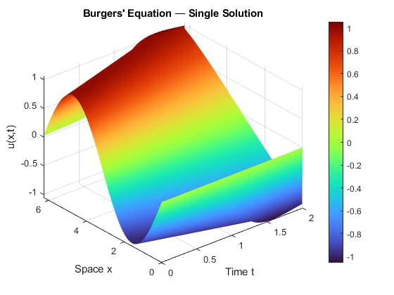
A Toy Example: Burgers’ Equation

Before going deeper, it helps to make the contrast concrete. Consider the 1D viscous Burgers’ equation:

uₜ + u · uₓ = ν · uₓₓ

It’s nonlinear, produces sharp gradients at low viscosity, and is a standard benchmark in both the PINN and neural operator literature. Simple enough to solve in a few lines of Python, interesting enough to reveal real challenges.

The PINN workflow trains a neural network u(x, t; θ) for one specific choice of viscosity ν, initial condition u(x, 0), and boundary conditions, penalizing the PDE residual at scattered collocation points. The result is a single solution surface. Change ν or the initial condition, and you retrain from scratch.

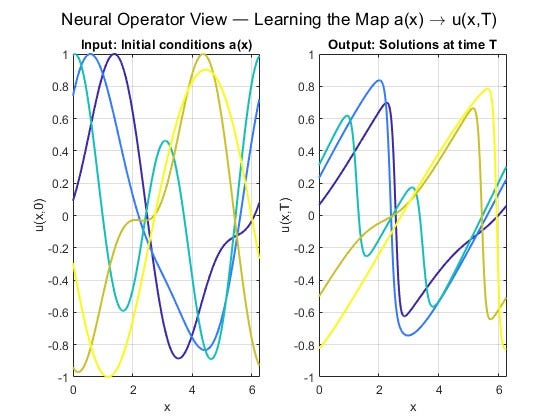
The neural operator workflow generates many Burgers’ solutions from a classical solver, each with a different initial condition, and trains a model to learn the map from input function a(x) to solution u(x, T) at a later time. The result is a reusable surrogate: given any new initial condition from that family, it predicts the solution in a single forward pass.

This is the core tradeoff in a picture: depth and physical fidelity for one problem, versus breadth and reusability across many.

Burgers’ equation solution surface for ν = 0.005, starting from u(x,0) = −sin(x). This is what a PINN trains to approximate, one specific trajectory, for one viscosity, one initial condition. The shock formation visible at later times is precisely what makes this a challenging benchmark for gradient-based training. Source: Author’s simulation.

The neural operator view. Left: five smooth initial conditions drawn from a random trigonometric family. Right: their corresponding solutions at time T = 2.0, produced by a classical finite-difference solver. A neural operator trains on pairs like these and learns to map any new a(x) to u(x,T) without re-solving the PDE generalizing across the entire family in a single forward pass. Source: Author’s simulation.

The classical solver this PINN would replace looks like this:

nu, Nx, Nt = 0.005, 256, 2000
dx, dt     = 2*np.pi/Nx, 2.0/Nt
x          = np.linspace(0, 2*np.pi, Nx, endpoint=False)
u          = -np.sin(x)   # initial condition

for n in range(Nt):
    uR   = np.roll(u, -1)
    uL   = np.roll(u,  1)
    fx   = (0.5*uR**2 - 0.5*uL**2) / (2*dx)  # conservative flux
    u_xx = (uR - 2*u + uL) / dx**2             # diffusion
    u    = u + dt * (-fx + nu * u_xx)

A trained PINN returns u(x,t) for any (x,t) in the domain without this loop, but only for this ν and this initial condition. A neural operator skips the loop entirely at inference time, and generalizes across the whole family.

Part I: Physics-Informed Neural Networks

PINNs, popularized by Raissi, Perdikaris, and Karniadakis in 2019, take a direct approach. You train a neural network u(x, t; θ) to approximate the solution of a PDE by penalizing it for violating the governing equation right in the loss function:

ℒ(θ) = λ_r · ‖N[u](x,t)‖² ← residual (PDE violation)
+ λ_bc · ‖u − g‖² ← boundary conditions
+ λ_d · ‖u − u_data‖² ← (optional) data term

where N[u] = ∂u/∂t + u·∇u − ν∇²u (e.g., Navier-Stokes)

The residual term is computed using automatic differentiation. PyTorch or JAX computes ∂u/∂x, ∂²u/∂x² etc. exactly through the network. No discretization grid is needed. You scatter “collocation points” in the domain and evaluate the PDE residual there.

What PINNs are good at

PINNs shine in a specific niche: inverse problems and sparse data regimes. Suppose you have scattered sensor measurements of a flow field, and you want to recover pressure, viscosity, or source terms you never directly observed. PINNs handle this elegantly: you add the data as a soft constraint while the PDE regularizes the solution space. This combination is hard to replicate with classical methods.

They also handle irregular geometries gracefully, since collocation points can be placed anywhere without a mesh. And they can operate with no training data at all, deriving everything from the equation itself.

Where PINNs win: inverse problems · parameter identification · mixed physics-data scenarios · small domains · irregular boundaries · when you have one specific problem to solve, not a family of them.

The PINN pain points

PINNs have real, well-documented failure modes. The loss landscape is notoriously difficult to optimize. The interplay between residual, boundary, and data terms creates competing gradients. The spectral bias of neural networks means they learn low-frequency components of the solution first, struggling with sharp gradients or multiscale dynamics.

There is, however, one often-overlooked advantage in how PINNs fail: they fail visibly. When a PINN produces a poor solution, the PDE residual is high and you can see it. You can plot the residual across the domain and know exactly where the model is struggling. This built-in diagnostic is easy to take for granted, until you work with methods that lack it.

More fundamentally: PINNs solve one problem at a time. Train a PINN for ν = 0.01 viscosity, and it tells you nothing about ν = 0.001. Every new initial condition, boundary condition, or parameter setting requires a full retraining from scratch. This is a critical limitation.

Part II: Neural Operators

Neural operators, developed primarily through the work of Kovachki, Li, Anandkumar and collaborators at Caltech, start from a different question entirely. Instead of asking “what is u(x,t) for this equation with these conditions?”, they ask:

Can we learn the solution operator itself, the mapping from any initial condition to any output, in a single training run?

In mathematical terms, a neural operator learns a map G†: A → U, where A is a function space of inputs (initial conditions, forcing terms, coefficients) and U is a function space of outputs (solutions). This is a map between infinite-dimensional function spaces, not between finite-dimensional vectors.

G†(a)(x) ≈ u(x)

where: a ∈ A is the input function (e.g., initial condition); u ∈ U is the output function (e.g., solution at time T); x can be ANY point in the domain. Key: trained once, evaluates instantly for ANY new a, on ANY discretization.

The Fourier Neural Operator (FNO)

The most influential architecture is the Fourier Neural Operator (FNO), introduced by Li et al. in 2020. It applies learned linear transforms in Fourier space, capturing global, long-range dependencies efficiently, then combines them with local nonlinear transforms. The result is a model that can generalize across discretizations under favorable conditions: train it on a 64×64 grid, and in many settings evaluate it on 256×256, though the degree of resolution transfer depends on the problem structure, data representation, and how far the target resolution departs from training.

On standard Navier–Stokes benchmarks, FNO demonstrated substantial speedups over traditional solvers while maintaining competitive accuracy. In atmospheric modeling, architectures in this family, such as Pathak et al.’s FourCastNet, have shown the ability to run medium-range weather forecasts in seconds rather than the minutes required by conventional numerical models, though accuracy comparisons are highly benchmark-dependent and the AI weather modeling landscape has evolved rapidly since FourCastNet’s publication.

Where neural operators win: parametric families of PDEs · design sweeps · real-time simulation · large-scale surrogates · when you need to solve the same PDE type many times with different inputs.

The cost of generality

Neural operators require training data, and lots of it. You typically generate thousands of (input, solution) pairs from a classical solver, then train the operator to mimic that mapping. This means paying the compute cost upfront. It also creates a dependency worth naming explicitly: the training data comes from the very classical solvers that neural operators are supposed to accelerate. Neural operators don’t eliminate traditional solvers. They amortize their cost, spreading the expense of many classical solves across a reusable model that handles future queries cheaply. Whether that tradeoff pays off depends on how many forward solves you ultimately need.

There’s a subtler and more dangerous limitation: neural operators are powerful only when your test problems resemble your training distribution. If the initial conditions, parameter ranges, or forcing terms at inference time fall outside what the model saw during training, performance can degrade, sometimes silently. Unlike a PINN, where a high PDE residual tells you the model is struggling, a neural operator can produce confident but physically meaningless outputs with no built-in warning. This asymmetry in failure transparency is one of the most important practical distinctions between the two paradigms, and it means that deploying neural operators responsibly requires careful out-of-distribution monitoring. Generalization across PDE types is also limited; a neural operator trained on Navier–Stokes won’t transfer to elasticity.

Head-to-Head

Practical tradeoffs across key dimensions. The right choice depends on the workload, not the architecture. Source: Author’s analysis based on Raissi et al. (2019), Li et al. (2020), Lu et al. (2021).

The Synthesis: Physics-Informed Neural Operators

The research frontier has moved toward combining both ideas. Physics-Informed Neural Operators (PINOs) train neural operators with both data and PDE residual constraints, getting generalization from the operator structure while using the physics to regularize and reduce data requirements.

The intuition behind the hybrid approach is elegant. The operator architecture, typically FNO, provides a strong structural prior: it learns a basis of solution modes from data, giving the optimizer a dramatically better starting point than a randomly initialized PINN. The physics loss then fine-tunes accuracy without requiring more solver data. Crucially, PINO can operate at multiple resolutions: training on coarse-resolution data (which is cheap to generate) while imposing PDE constraints at a finer resolution. This multi-resolution strategy yields high-fidelity reconstructions without the cost of generating high-resolution training data, and it sidesteps the optimization difficulties that plague PINNs on challenging problems like multi-scale Kolmogorov flows.

In several benchmark studies, this hybrid approach has outperformed either method alone, particularly in low-data regimes where pure neural operators lack sufficient training signal and pure PINNs struggle to converge.

DeepONet (Lu et al., 2021) offers a complementary operator-learning paradigm. Its branch-trunk architecture separates the encoding of input functions from the evaluation of output fields, and this structure integrates more naturally with the PINN loss framework than FNO does. This makes DeepONet particularly well-suited for physics-constrained operator learning in inverse problems, where you want both the generalization of an operator and the physical guardrails of a PDE loss. The boundary between the two approaches is already blurring as the field matures.

The Verdict

PINNs and neural operators are not replacements for one another so much as different abstractions for different scientific workloads. One embeds physics into the solution of a specific problem; the other amortizes solution over a family of problems.
If your problem is inverse, data-sparse, and tightly constrained by known physics, PINNs are often the natural starting point. If your goal is repeated fast forward solves across a broad family of inputs, neural operators are usually the more scalable abstraction. And if you need both generalization and physical structure, the most promising direction is increasingly hybrid.
What neither approach is, yet, is a drop-in replacement for a classical solver in high-stakes settings. Both fail in predictable ways, and the practitioner who understands those failure modes will always outperform the one who doesn’t.