Why Recommendation Systems Are Structurally Different from Deep Learning[1/2]

digitado ⋅ 19 de January de 2026

Why One-Hot Features and Naïve MLPs Fail

This article is Part 1 of a two-part series on why recommendation systems require fundamentally different modeling assumptions from standard deep learning.

📌 TL;DR

Recommendation systems are not just another application of deep learning. Their core difficulty does not come from model depth or data scale, but from the structure of the problem itself: massive sparsity, discrete identities, and relational signals that do not fit naturally into standard neural networks.

This article explains why naïvely applying MLPs to sparse ID features fails, how embeddings emerged as a necessary structural fix, and why recommendation systems should be understood as relationship modeling problems, not generic function approximation tasks.

The reference paper: https://arxiv.org/pdf/1906.00091

1. Why Are Recommendation Systems an “Odd One Out” in Deep Learning?

In almost all large internet companies, recommendation and personalization systems occupy a core position in the business.

Among them, the most typical and representative task is CTR (Click-Through Rate) prediction. However, from the very beginning, the modeling perspective of recommendation systems was not designed for neural networks. On the contrary, recommendation systems are arguably the most awkward branch within deep learning.

Two Completely Different Origins of Thought

The deep learning recommendation models we see today did not naturally evolve along a single path.

Instead, they are the result of two almost independently developed lines of thought, which were forcibly merged under industrial demands. Understanding the differences between these two paths is a prerequisite for understanding DLRM.

1.1 Path One: The “Recommendation System” Perspective — Relationship Modeling

The traditional recommendation system paradigm has never been primarily concerned with the regression function itself, but rather with a more fundamental question:

What kind of relational structure exists between users and items?

Early recommendation systems went through several stages:

Content-based filtering — Items are manually labeled, and users choose preferred tags.
Collaborative filtering — Based on users’ historical behaviors and similar users.
Matrix factorization / latent factor methods

Users and items are mapped into a latent space, and preferences are modeled via vector relationships.

In these models, users and items themselves are discrete “identities”:

user_id
item_id

In later matrix factorization models, the core objective is:

To learn a comparable position (latent factor / embedding) for each discrete identity.

An intuitive illustration of latent factors (embeddings) in recommendation systems:

This classic illustration from Matrix Factorization Techniques for Recommender Systems (2009) shows that users and movies are no longer treated as high-dimensional sparse IDs or rating records, but are instead mapped together into a shared low-dimensional vector space.

The two axes in the figure (for example, serious–escapist) are not manually defined features, but latent factors automatically learned by the model from user behavior data.

This representation reveals the core idea of matrix factorization models:

Users with similar preferences cluster in nearby regions of the space
Movies with similar semantics naturally form clusters
The inner product or distance between a user and a movie characterizes their degree of match

It is important to emphasize that in this paradigm:

Embeddings are not an input preprocessing trick, but the core parameterization of the model itself.

Recommendation systems are not focused on predicting an exact rating, but on modeling the relational structure between discrete entities.

It is precisely this latent factor idea that formed the theoretical foundation for the widespread adoption of embedding methods in recommendation systems, and directly influenced the design of modern deep recommendation models, including DLRM.

1.2 Path Two: The “Predictive Analytics” Perspective — Function Approximation

The second path originates from statistical learning and predictive analytics. The starting point of this path is very straightforward, for example:

Given features such as user age, time, and price, predict whether an advertisement will be clicked (CTR).

This corresponds to the typical evolution:

Logistic Regression
→ More complex nonlinear models
→ MLP / deep neural networks

In this path, the problem is naturally modeled as: y = f(x)

with the implicit assumptions that:

Features are numerical
The feature space is continuous
The model’s task is to approximate a complex function

When this approach begins to face discrete features, it encounters fundamental conflicts:

Discrete features cannot directly enter continuous models
One-hot / multi-hot encoding leads to dimensional explosion

As a result, embeddings are introduced as an engineering technique.

In this path:

Embeddings serve the MLP as an intermediate representation
The goal is to translate a “discrete problem” into a “continuous problem”
The core task remains regression / classification

The “translation process” of discrete features in the predictive analytics pipeline:

It is precisely in this process that the tension between the predictive analytics path and the traditional recommendation system path gradually emerges:

The former focuses on function approximation
The latter focuses on relational structures between discrete entities

This difference is exactly the problem that DLRM attempts to systematically resolve.

1.3 The Starting Point of DLRM: Fusion, Not Replacement

Under this tension, DLRM provides its own answer:

“A personalization model that was conceived by the union of the two perspectives described above.”

DLRM’s design is not simply “applying MLPs to recommendation systems”, but instead:

Treating discrete features in the way recommendation systems do
Treating continuous features in the way deep learning (MLPs) does
Explicitly modeling structured interactions between features in between

If traditional recommendation systems excel at answering “who is similar to whom”, and deep learning excels at answering “what happens given these features”, then DLRM asks:

How can we simultaneously model relationships between discrete entities and nonlinear expressions of continuous features?

2. Why Sparse Features and MLPs Are Fundamentally Mismatched

2.1 Starting from the Most Naïve CTR Modeling Attempt

We begin from the most realistic and most common engineering starting point.

The target is a standard CTR task: predicting whether a user will click on an advertisement at a given moment.

Assume that a single impression contains the following information:

user_id: the current user
item_id: the displayed advertisement
hour: the display time
price: the advertisement price
historical_ctr: historical statistical features

A very natural modeling idea is:

Concatenate all these features,
Feed them into a multilayer perceptron (MLP),
Output the click probability.

Formally, this can be written as:

where x is the concatenation of all features.

This model is entirely based on the predictive analytics perspective, treating CTR as a standard binary classification / regression problem.

In the early stages of many systems, this is indeed the first implemented and easiest-to-deploy solution.

2.2 “Sparsity” in Recommendation Systems: Where the Problems Begin

The real problems arise at the feature representation stage. In CTR scenarios, the most informative features are precisely categorical identity features:

user_id
item_id
…

These features share several typical characteristics:

Extremely large cardinality (millions or even billions)
Each sample only activates a very small number of values
IDs themselves have no numerical magnitude semantics

The most straightforward engineering approach is to use one-hot or multi-hot encoding. But what does this imply?

Each sample only activates a very small number of coordinates in an extremely high-dimensional input space.

When such inputs enter the first layer of an MLP, the problem immediately becomes apparent.

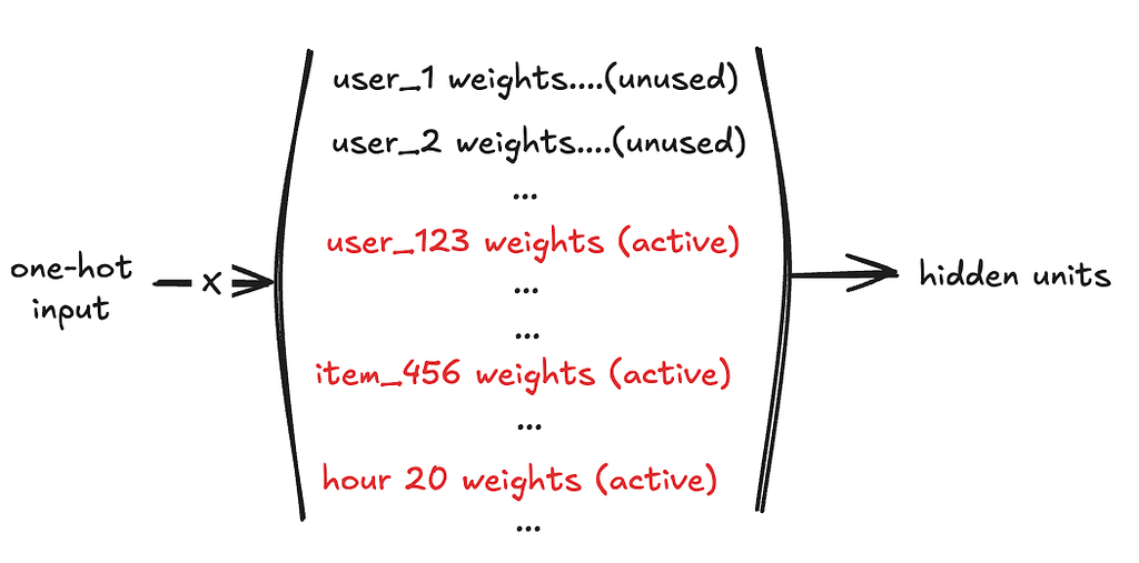
Naïve MLP architecture: all features are directly used as numerical inputs, passed through several fully connected layers with ReLU activations, and finally through a Sigmoid to output the click probability:

In this structure: Each row of the first-layer weight matrix corresponds to a specific ID(some user, item, or hour), For a single sample:

Only the rows corresponding touser_id = 123, item_id = 456, hour = 20are actually used
The vast majority of parameters receive no gradient at all for this sample

From an effect perspective, this is equivalent to:

The model memorizing an entire independent row of parameters for each ID, instead of learning a shared, generalizable structure
The parameter size is enormous, but each sample only updates a tiny fraction of parameters, resulting in extremely low learning efficiency

2.3 The Second Problem: The Model Almost Has No Concept of “Similarity”

A deeper issue lies in generalization ability.

Under one-hot representations, as long as two IDs are different, they are completely orthogonal in the input space.

This means that even if item_A and item_B are highly similar in semantics, content, and user groups, they are entirely unrelated in the model’s eyes.

If we want the model to understand:

“Does this user match this advertisement?”

Then in a one-hot + MLP structure, the only hope is that: The MLP implicitly learns some kind of higher-order combination relationships in later layers

Naïve MLP architecture: the first-layer weight matrix of an MLP under one-hot inputs:

In theory, this requires the model to learn second-order or even higher-order interactions.

However, if we explicitly model second-order interactions, the parameter size quickly becomes uncontrollable. For example, suppose there are N discrete features, each mapped to a d-dimensional representation. The number of explicit second-order interaction terms is:

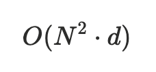
At the feature scale typical of recommendation systems, this is almost infeasible in practice.

As a result, the MLP is forced to take on a task it is inherently not good at:

Guessing relationships between features from sparse, orthogonal inputs without any structural assumptions.

3. Embeddings: A Unified Representation from Collaborative Filtering to Neural Networks

3.1 The Essence of Embeddings: From Discrete Identities to a Continuous Geometric Space

The essence of embeddings is to map discrete identities into a continuous geometric space.

From a computational perspective, an embedding is essentially a learnable lookup operation:

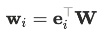
where:

e_i^T is a one-hot vector (used only for indexing)
W is the embedding table
w_i is the embedding vector corresponding to the ID

In the multi-hot scenario (for example, user interest tags), this process naturally generalizes to a weighted sum:

Here is a very important but often overlooked fact:

The embedding table itself is a model parameter, but it does not participate in dense computation; instead, it is “looked up” and used.

This distinction directly determines the scalability of subsequent models.

3.2 The First Model Upgrade: From One-Hot + MLP to Embedding + MLP

In Chapter 2, we analyzed the structural problems of one-hot + MLP from an engineering perspective:

Enormous parameter size
Extremely low learning efficiency
A complete lack of any notion of “similarity”

A most natural improvement idea is therefore:

Keep the overall MLP structure unchanged, and simply replace one-hot features with embeddings.

Core Structural Change of Embedding + MLP

In CTR scenarios, the model structure can be upgraded to the following form:

Each discrete feature has its own embedding table, and
The embedding vectors are concatenated together with dense features and fed into the MLP.

At this point, a crucial structural change occurs:

The number of IDs no longer directly enters the MLP.

Core structure of embedding + MLP: one-hot lookup followed by embedding tables:

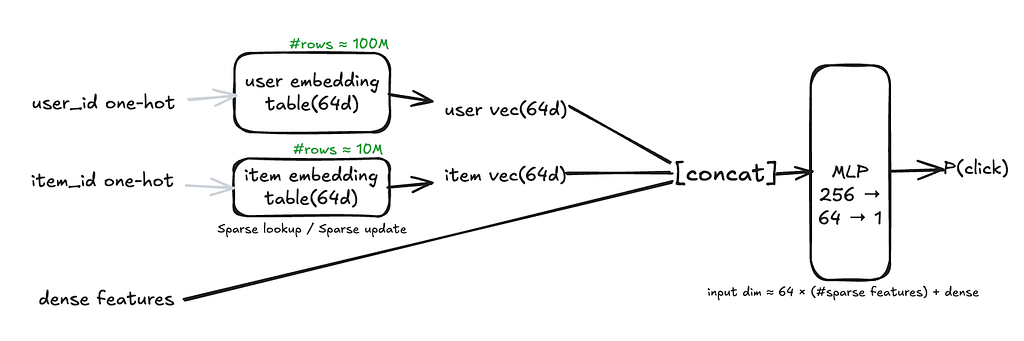
This diagram fully illustrates the core structure of embedding + MLP:

user_id one-hot → user embedding table (64d), Number of rows ≈ (10⁸), Sparse lookup / sparse update
item_id one-hot → item embedding table (64d), Number of rows ≈ (10⁷)

The resulting: user vector (64d), item vector (64d), together with dense features are concatenated and fed into an MLP with a small parameter size.

At this point, the MLP input dimension becomes:

This means:

The parameter scale of the MLP is now completely decoupled from the number of users and ads.

3.3 Where Did the Parameters Go?

When I reached this point while reading the paper, I had a question: The embedding tables themselves still contain billions of parameters.Does this really count as an “improvement”?

The answer is:

This is a structural improvement, not merely a reduction in parameters

The key difference lies in how parameters are used.

Characteristics of MLP weights:

Used by every sample
Dense computation
Participate in forward and backward propagation at every layer
Must reside on accelerators

Characteristics of embedding tables:

Each sample accesses only a very small number of rows
Updates are sparse
Can be stored in a distributed manner
Behave more like the model’s learnable memory

Therefore, embedding tables are not “function parameters”, but rather a form of memory capacity that recommendation systems must possess.

The role of embeddings is not to eliminate parameter sizes that grow linearly with the number of IDs, but to:

Move these parameters from dense MLP weights into locations that are engineering-controllable.

3.4 What Embeddings Solve — and What They Do Not

At this point, we can give a clear summary of embeddings:

They alleviate the high-dimensional sparsity caused by discrete features
They break the orthogonal isolation between features under one-hot representations
They map users, items, and other discrete attributes into a unified continuous vector space

However, embeddings themselves only answer “how to represent features”, not “how features should interact.”

If the model structure remains:

embedding -> concat -> MLP

then:

Embeddings only serve as input representations for the MLP
Interactions between different features are still learned implicitly by the network
Whether the model captures reasonable feature combinations depends entirely on data and network capacity

From a modeling perspective, such a model is still essentially a generic function approximator, lacking an explicit inductive bias for feature interaction structures.

It is precisely here that the limitations of embedding-based approaches in structural modeling become apparent.

At this point, embeddings have solved an essential problem:

they provide a scalable way to represent discrete identities in a continuous space, breaking the orthogonality imposed by one-hot features.

But an important question remains unanswered:

Embeddings tell us how to represent features, not how those features should interact.

If all embeddings are simply concatenated and passed to an MLP,

then relationships between users, items, and contexts are still left to be discovered implicitly by a black-box network — often inefficiently and unreliably.

In the next part, we will see why this is not enough, and how structured interaction modeling — from Factorization Machines to DLRM — addresses this missing piece.

Why Recommendation Systems Are Structurally Different from Deep Learning[1/2] was originally published in Towards AI on Medium, where people are continuing the conversation by highlighting and responding to this story.

Like 0

Liked Liked