
Why My PyTorch Diffusion Model Was Slow — and How I Made It 3× Faster

Training a Diffusion Model — even on a “simple” dataset like MNIST — is a trial by fire for your hardware. You expect the GPU to do the heavy lifting, but more often than not, your expensive silicon is sitting idle, waiting for a sluggish pipeline to throw it a bone.
I recently took a DDPM (Denoising Diffusion Probabilistic Model) U-Net and put it through a rigorous optimization gauntlet. What started as a sluggish 3 minute and 10 second epoch ended in a lightning-fast 1 minute and 9 seconds (stabilizing at 1:15 under thermal load).
This is a ~60% speedup. Here is the detective story of how I hunted down the bottlenecks and crushed them in five distinct phases.
Code: 👉 Diffusion Model Optimization (Code)
The Pre-Flight Check: The Cloud I/O Trap
Before the first epoch even began, I walked right into a massive bottleneck regarding cloud data management in Google Colab.
Initially, I considered uploading the unzipped dataset folder directly to Google Drive, or uploading the ZIP and extracting it directly into the mounted Drive. Do not do this. It presents two agonizing problems:
- Transfer Latency: Uploading or extracting 60,000 individual small files to a cloud drive takes forever because of the massive overhead of creating thousands of file metadata entries over a network.
- Access Latency: Accessing images from a mounted Drive one-by-one during training is brutal. Every “read” request must travel over the network, turning millisecond disk reads into a process that takes hours.
The Fix: I uploaded a single, compressed ZIP file to Google Drive, but copied and extracted it directly into Colab’s local runtime environment (/content/). This reduced a multi-hour data-prep nightmare to just a few seconds, ensuring the training loop accessed files directly from local SSD storage.
The Baseline & The “More Batch Size” Delusion
The Setup: 2-core CPU, 15 GB GPU (Google Colab T4, 68 Streaming Multiprocessors).
The Stats: 3:10 per epoch with a batch size of 64. VRAM usage was hovering around 5GB
Like any reasonable engineer with spare VRAM, I thought: “If I just double the batch size to 128, the GPU will process more at once and finish faster.”
The Reality Check: The time didn’t budge. Not by a single second.
The Diagnosis: I was I/O Bound. With only 2 CPU cores, the process of reading images from the local disk and preprocessing them couldn’t keep up. The GPU would finish its math in milliseconds, then sit around twiddling its thumbs while the CPU gasped for air. Increasing the batch size just made the CPU work harder, keeping the GPU waiting even longer. However, because a larger batch size provides smoother, more stable gradient updates during training, I decided to keep batch_size=128 and set out to fix the actual data pipeline to support it.
Phase 1: Bypassing the Disk (The I/O Fix)
To stop the CPU from being the bottleneck, I had to stop it from touching the disk during the training loop entirely.
The Strategy: 1. RAM Pre-loading: I rewrote the Dataset class to perform a “one-time hit.” Instead of opening images during the training loop, I loaded all 60,000 images into system RAM as tensors during initialization.
The Anatomy of a Transfer: How RAM and the GPU Talk
To understand why data loading is so tricky, you have to look at the motherboard. Your system RAM (where the CPU lives) and your VRAM (where the GPU lives) are physically separated by the PCIe (Peripheral Component Interconnect Express) bus.
Think of system RAM as a massive warehouse, the GPU as a high-speed factory, and the PCIe bus as the highway connecting them. By default, standard system RAM is “pageable” — meaning the operating system is allowed to shuffle data around or page it out to the hard drive if it needs space. The GPU cannot safely pull data from pageable memory because the OS might move it mid-transfer.
So, the CPU normally has to do a hidden, expensive chore: it copies the batch of images from pageable memory into a temporary “locked” staging area, and then sends it down the PCIe highway.
The Asynchronous Fix: pin_memory and non_blocking
We can eliminate that hidden CPU chore by using two simple commands, combined with pre-loading our dataset.
- pin_memory=True (In the DataLoader): This tells PyTorch to allocate our batches directly into “page-locked” (pinned) memory from the start. The OS is forbidden from moving it. This allows the GPU to use Direct Memory Access (DMA) to securely pull the data across the highway, completely bypassing the CPU’s staging process.
- non_blocking=True (In the .to(device) call): Normally, the Python script freezes and waits for the PCIe transfer to finish. non_blocking=True makes it an asynchronous fire-and-forget command. The CPU fires data down the highway and instantly goes back to preparing the next batch while the GPU crunches the current batch.
def load_images(self, im_path):
    assert os.path.exists(im_path), f"images path {im_path} does not exist"
    ims, labels = [], []
    to_tensor = torchvision.transforms.ToTensor()

    print(f"Pre-loading {self.split} images into RAM...")
    for d_name in tqdm(os.listdir(im_path)):
        for fname in glob.glob(os.path.join(im_path, d_name, f'*.{self.im_ext}')):
            # THE CURE: Load and process once during initialization
            im = Image.open(fname)
            im_tensor = to_tensor(im)
            im_tensor = (2 * im_tensor) - 1
            ims.append(im_tensor)
            labels.append(int(d_name))

    return ims, labels

def __getitem__(self, index):
    # Immediate return directly from RAM
    return self.images[index]
The Result: Epoch time dropped to 2:57. It wasn’t a big jump, but it was the fundamental cure. It proved the pipeline was no longer I/O bound. We were finally Compute Bound.
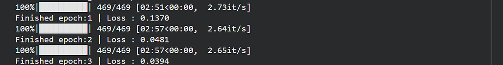
The first epoch is slightly faster (~2:51) due to initial caching/warm-up effects, after which training stabilizes at ~2:57 per epoch.
Phase 2: Shrinking the Math (The AMP Upgrade)
Now that the data was arriving like a firehose, I had to make the math more efficient. By default, PyTorch uses FP32 (32-bit floating point). But modern GPUs have Tensor Cores specifically designed to crush FP16 math.
I implemented Automatic Mixed Precision (AMP) using autocast and a GradScaler.
How autocast Acts Like a Traffic Cop
Not all math is created equal. autocast has a hardcoded, under-the-hood list of PyTorch operations:
- The FP16 Safe Zone: For heavy lifting like matrix multiplications (Linear, Conv2d), autocast instantly casts the tensors down to 16-bit. These operations are highly parallelizable and don’t need infinite decimal precision.
- The FP32 Danger Zone: For operations where precision is critical to prevent numerical collapse — like Softmax, BatchNorm, or calculating the final Loss — autocast strictly leaves them in 32-bit.
Saving the Gradients (GradScaler)
16-bit floats have a fatal flaw: they cannot represent extremely tiny numbers. In Deep Learning, gradients shrink as the model converges. If a gradient rounds down to zero, the model stops learning entirely — a phenomenon called Gradient Underflow.
This is why we use GradScaler. Before doing the backward pass, the scaler multiplies the loss by a massive number. This artificially “inflates” the gradients so they safely stay within the FP16 representable range during the math. Once the backward pass is done, it un-scales the gradients back to their normal, tiny size right before updating the optimizer.
from torch.cuda.amp import autocast, GradScaler
scaler = GradScaler()
for data, target in dataloader:
    optimizer.zero_grad()
    with autocast(): # Runs operations in FP16 where safe
        output = model(data, t)
        loss = criterion(output, target)
    scaler.scale(loss).backward()
    scaler.step(optimizer)
    scaler.update()
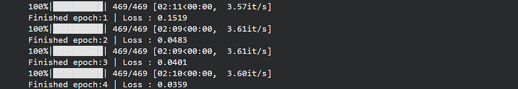
The Result: A massive breakthrough. The time plummeted to 2:10. By using half the precision, we engaged the Tensor Cores and effectively doubled the throughput of the GPU’s arithmetic units.
Phase 3: The VRAM Revelation
A brilliant side effect of AMP is that 16-bit tensors take up half the space. My VRAM usage tanked.
I took that extra “room” and finally did what I tried at the very beginning: I increased the batch size from 128 to 192. This pushed my VRAM consumption to a very healthy 11.2 GB out of 15 GB.
The Result: The epoch time dropped to 2:03. Because the I/O bottleneck was dead, the larger batch size actually allowed the GPU to saturate its 68 SMs effectively.
Phase 4: The Nuclear Option (torch.compile)
By default, PyTorch operates in “Eager Mode.” It reads your code line-by-line via Python. If your model says x = x + 1 and then x = x * 2, the GPU has to read x from VRAM, add 1, write it back to VRAM, read it again, multiply by 2, and write it back again. This memory read/write overhead is deadly.
The Kernel Fusion Wizard
Introduced in PyTorch 2.0, torch.compile abandons Eager Mode. Before any training happens, it does a “dry run” to capture your entire computational graph. It performs Kernel Fusion: it looks at that x + 1 and x * 2 and fuses them into a single, highly optimized GPU micro-program. The GPU now reads x from memory once, does all the math in its ultra-fast on-chip cache, and writes it back once.
Where to write it: You must compile the model after moving it to the GPU, but before passing its parameters to the optimizer.
# 1. Instantiate the model
model = UNet().to(device)
# 2. Compile it (The Nuclear Option)
model = torch.compile(model)
# 3. Pass the COMPILED model's parameters to the optimizer
optimizer = torch.optim.AdamW(model.parameters(), lr=1e-4)
The Graph Recompilation Trap
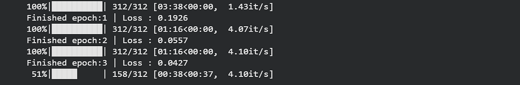
When I fired this up, the first epoch took an agonizing 6 minutes. Subsequent epochs dropped to 1:09. What happened?

I had forgotten about the “uneven batch.” My dataset size didn’t divide perfectly by 192, leaving a smaller batch at the very end of the epoch. The compiler optimized the network for a batch of 192, but when that final tiny batch hit, the compiler panicked. It threw away its work and triggered a massive recompilation to account for the new shape.
The Fix: I added drop_last=True to the DataLoader so the shape remained completely static.
The Result: The recompilation stall vanished. The first-epoch compilation overhead dropped from 6 minutes to 3 minutes, and every single epoch after that plummeted to an incredible 1:09.

Phase 5: Sustained Performance Under Load
In a vacuum, 1:09 is the absolute speed limit of this setup. But real hardware doesn’t operate in isolation. After repeated training sessions, reconnects, and extended usage over hours, performance began to drift.
The same setup that initially ran at 1:09 would later stabilize around ~1:15 per epoch — not due to a single warm-up phase, but as a result of sustained load and session-level variability. Interestingly, rerunning the experiment fresh the next day brought the time back to ~1:09, where it remained stable for the whole training.
Final Outcome: By systematically hunting down bottlenecks, I reduced the total training time for 40 epochs strictly under 50 minutes.

In a clean, uninterrupted run, the model consistently maintains ~1:09 per epoch. The ~1:15 regime emerges only after extended usage across multiple sessions.
Optimization isn’t about one big trick — it’s about systematically removing bottlenecks until the hardware can finally do what it was meant to.
But speed is only half the story. In Part 2, I’ll dive into the inference results — what the model actually generates, and whether these optimizations hold up in practice.
The complete implementation, experiments, and optimizations are available here:
👉 Diffusion Model Optimization (Code)
If you found this helpful, consider leaving a clap👏 — it helps others discover the article.
Thanks for reading! Part 2 coming soon.
References
- DDPM Research Paper
- DDPM (Denoising Diffusion Probabilistic Models) lecture playlists and tutorials
- Andrej Karpathy, Let’s Reproduce GPT-2 — insights on training and optimization
Why My PyTorch Diffusion Model Was Slow — and How I Made It 3× Faster was originally published in Towards AI on Medium, where people are continuing the conversation by highlighting and responding to this story.