
What Happens When a GPT Reads Your Message
The role of embeddings in how LLMs turn your words into numbers, and why those numbers capture meaning.
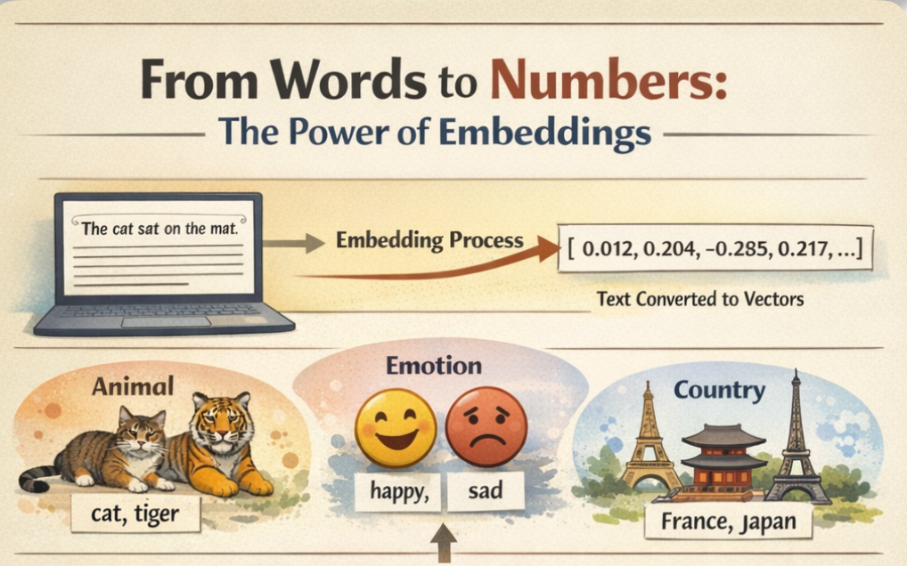
Large language models do not read words. They read numbers. Every word, every sentence, every paragraph that flows through a model like GPT-5 or LLaMA is first converted into a dense numerical representation called an embedding. That conversion is not a formality. It is where meaning begins.
This article is part of a series on Generative AI. The previous articles covered the overview of the Encoder architecture and how transformers process and represent input. But before any of that can happen, raw text has to become something a model can actually work with. That’s where embeddings come in. They are the foundation layer, the step that converts language into numbers before attention, generation, or reasoning can begin.
The Core Problem: Machines Cannot Read
A computer has no concept of what the word “cat” means. It does not know that a cat is small, furry, and uninterested in your schedule. All it has is the character sequence c-a-t.
Early approaches in NLP tried to solve this with simple encodings. One-hot encoding, for example, assigns each word a unique binary vector. In a vocabulary of 10,000 words, “cat” might be represented as a vector with a 1 in position 4,237 and 0 everywhere else. This works mechanically, but it captures nothing about meaning. Under one-hot encoding, “cat” is equally distant from “kitten” as it is from “democracy.” There is no notion of similarity, no relationships, no context.
Embeddings solve this by placing words in a continuous vector space where proximity reflects meaning. Words that are used in similar contexts end up near each other. Words with different meanings end up far apart. And, most remarkably, the directions in this space encode relationships.
From Words to Vectors: The Intuition
Think of it this way. Suppose every word in the English language could be described along a set of hidden dimensions, how “alive” something is, how “large” it is, how “abstract” it is, whether it relates to emotion, motion, food, and so on.
An embedding is essentially a position along hundreds of these dimensions. The word “cat” might score high on “alive,” medium on “size,” and low on “abstract.” The word “philosophy” would score the opposite. The word “tiger” would land somewhere near “cat” along most dimensions but diverge on “size” and “danger.”
No one manually defines these dimensions. The model learns them from data, from seeing millions of sentences and learning which words appear in similar contexts. The result is a dense vector (typically 100 to 1,000+ numbers) for each word that captures its semantic fingerprint.
Seeing It in Code
The easiest way to understand embeddings is to work with them. The gensim library provides pre-trained Word2Vec embeddings that demonstrate the core concepts clearly.
import gensim.downloader as api
import numpy as np
# Load pre-trained Word2Vec embeddings (trained on Google News, 3 million words)
model = api.load("word2vec-google-news-300")
# Each word is now a 300-dimensional vector
cat_vector = model["cat"]
print(f"Dimensions: {cat_vector.shape}")
print(f"First 10 values: {cat_vector[:10]}")
[==================================================] 100.0% 1662.8/1662.8MB downloaded
Dimensions: (300,)
First 10 values: [ 0.0123291   0.20410156 -0.28515625  0.21679688  0.11816406  0.08300781
  0.04980469 -0.00952148  0.22070312 -0.12597656]
Three hundred numbers. That is what “cat” looks like to a machine. Not a picture, not a definition, a coordinate in 300-dimensional space.
Similarity: Distance Reflects Meaning
If embeddings are meaningful, then similar words should be close together. This can be tested directly using cosine similarity, a measure of how aligned two vectors are, regardless of their magnitude.
# Words that should be similar
pairs_similar = [("cat", "kitten"), ("car", "automobile"), ("happy", "joyful")]
# Words that should be dissimilar
pairs_different = [("cat", "democracy"), ("car", "philosophy"), ("happy", "concrete")]
print("Similar pairs:")
for w1, w2 in pairs_similar:
    sim = model.similarity(w1, w2)
    print(f"  {w1} ↔ {w2}: {sim:.3f}")
print("nDissimilar pairs:")
for w1, w2 in pairs_different:
    sim = model.similarity(w1, w2)
    print(f"  {w1} ↔ {w2}: {sim:.3f}")
Similar pairs:
  cat ↔ kitten: 0.746
  car ↔ automobile: 0.584
  happy ↔ joyful: 0.424
Dissimilar pairs:
  cat ↔ democracy: 0.104
  car ↔ philosophy: 0.062
  happy ↔ concrete: 0.047
The similar pairs will score in the range of 0.7 to 0.9. The dissimilar pairs will score near 0. The model was never told that a kitten is a young cat. It figured that out from how those words are used in text.
The Famous Arithmetic: King − Man + Woman = ?
The most celebrated property of embeddings is that they encode relationships as directions in space. The classic example:
# Analogy: king - man + woman = ?
result = model.most_similar(positive=["king", "woman"], negative=["man"], topn=3)
print("king - man + woman =")
for word, score in result:
    print(f"  {word}: {score:.3f}")
king - man + woman =
  queen: 0.712
  monarch: 0.619
  princess: 0.590
This works because the vector from “man” to “woman” encodes a gender direction. Subtracting “man” from “king” removes the male component, and adding “woman” lands near “queen.” The model learned this relationship purely from patterns in text, with no explicit knowledge of gender or royalty.
This property extends beyond toy examples:
# More analogies
analogies = [
    (["Paris", "Germany"], ["France"], "Capital relationships"),
    (["bigger", "cold"], ["big"], "Comparative forms"),
    (["walking", "swam"], ["walk"], "Tense transformation"),
]
for positive, negative, label in analogies:
    result = model.most_similar(positive=positive, negative=negative, topn=1)
    print(f"{label}: {result[0][0]} ({result[0][1]:.3f})")
Capital relationships: Berlin (0.764)
Comparative forms: colder (0.678)
Tense transformation: swum (0.619)
The embedding space is not a bag of numbers. It is a structured map of meaning, and directions on that map correspond to real-world relationships.
Visualizing the Embedding Space
Three hundred dimensions cannot be seen directly, but they can be projected down to two dimensions using t-SNE (used for dimensionality reduction). This collapses most of the structure, but the clusters that emerge are revealing.
from sklearn.manifold import TSNE
import matplotlib.pyplot as plt
# Select words from distinct categories
categories = {
    "Animals": ["cat", "dog", "tiger", "lion", "elephant", "rabbit", "wolf"],
    "Vehicles": ["car", "truck", "bus", "motorcycle", "bicycle", "airplane", "helicopter"],
    "Emotions": ["happy", "sad", "angry", "afraid", "excited", "calm", "anxious"],
    "Countries": ["India", "Germany", "Japan", "Brazil", "France", "Canada", "Australia"],
}
words = []
vectors = []
labels = []
for category, word_list in categories.items():
    for word in word_list:
        if word in model:
            words.append(word)
            vectors.append(model[word])
            labels.append(category)
vectors = np.array(vectors)
# Reduce to 2D
tsne = TSNE(n_components=2, random_state=42, perplexity=8)
vectors_2d = tsne.fit_transform(vectors)
# Plot
colors = {"Animals": "#e74c3c", "Vehicles": "#3498db", "Emotions": "#2ecc71", "Countries": "#f39c12"}
plt.figure(figsize=(12, 8))
for i, word in enumerate(words):
    color = colors[labels[i]]
    plt.scatter(vectors_2d[i, 0], vectors_2d[i, 1], c=color, s=100, edgecolors="k", linewidths=0.5)
    plt.annotate(word, (vectors_2d[i, 0] + 1, vectors_2d[i, 1] + 1), fontsize=9)
# Legend
for category, color in colors.items():
    plt.scatter([], [], c=color, s=100, label=category, edgecolors="k", linewidths=0.5)
plt.legend(fontsize=10)
plt.title("Word Embeddings Projected to 2D — Semantic Clusters Emerge")
plt.axis("off")
plt.tight_layout()
plt.savefig("embedding_clusters.png", dpi=150, bbox_inches="tight")
plt.show()

Animals cluster together. Vehicles cluster together. Countries cluster together. The model was never told these categories exist. The structure emerged from learning which words appear in similar contexts.
The Math Behind Embeddings
The code above demonstrates that embeddings work. This section explains why they work, in three core ideas.
1. Dot Product — Measuring Overlap
The simplest way to compare two vectors is the dot product: multiply corresponding elements and sum them up.

If two vectors point in roughly the same direction, the dot product is large and positive. If they point in opposite directions, it’s large and negative. If they are unrelated, it’s near zero.
# Manual dot product
cat = model["cat"]
kitten = model["kitten"]
democracy = model["democracy"]
dot_similar = np.dot(cat, kitten)
dot_different = np.dot(cat, democracy)
print(f"cat · kitten = {dot_similar:.2f}")
print(f"cat · democracy = {dot_different:.2f}")
cat · kitten = 7.65
cat · democracy = 1.14
The dot product for “cat” and “kitten” will be significantly higher than for “cat” and “democracy.” But there is a problem, longer vectors naturally produce larger dot products regardless of meaning. A word that just happens to have large values across all dimensions would score high against everything.
2. Cosine Similarity: Direction Over Magnitude
Cosine similarity fixes this by normalizing for vector length. It measures the angle between two vectors, not their magnitude.

The result is always between -1 (opposite) and 1 (identical direction). This is what model.similarity() computes, and it’s the standard similarity metric for embeddings.
from numpy.linalg import norm
def cosine_similarity(a, b):
    return np.dot(a, b) / (norm(a) * norm(b))
# Compare dot product vs cosine similarity
print("Dot product:")
print(f"  cat · kitten = {np.dot(cat, kitten):.2f}")
print(f"  cat · democracy = {np.dot(cat, democracy):.2f}")
print("nCosine similarity:")
print(f"  cat ↔ kitten = {cosine_similarity(cat, kitten):.3f}")
print(f"  cat ↔ democracy = {cosine_similarity(cat, democracy):.3f}")
Dot product:
  cat · kitten = 7.65
  cat · democracy = 1.14
Cosine similarity:
  cat ↔ kitten = 0.746
  cat ↔ democracy = 0.104
Cosine similarity strips away magnitude and asks a purer question: are these two words pointing in the same semantic direction?
3. How the Vectors Are Learned
The numbers inside an embedding are not assigned by hand. They are learned through training. Word2Vec’s Skip-gram model works by giving the network a word and asking it to predict the words that appear nearby in real text.
For example, given the sentence “the cat sat on the mat,” if the input word is “cat,” the model tries to predict “the,” “sat,” “on.” The network has a hidden layer, and the weights of that hidden layer become the embedding.
The training objective is simple: adjust the weights so that words appearing in similar contexts produce similar predictions. Over millions of sentences, words used in similar ways converge to similar vectors. “Cat” and “kitten” appear near the same words (pet, cute, furry), so their vectors drift together. “Cat” and “democracy” don’t share context, so their vectors stay apart.
No one defines the 300 dimensions. No one labels what each axis means. The structure emerges entirely from the patterns in language.
From Word Embeddings to LLM Embeddings
Word2Vec embeddings are static, the word “bank” gets the same vector whether the sentence is about finance or rivers. This is a fundamental limitation. Meaning depends on context.
Modern LLMs like GPT and BERT solve this with contextual embeddings. Instead of one fixed vector per word, the model produces a different vector for every occurrence of a word, shaped by the surrounding sentence.
from transformers import AutoTokenizer, AutoModel
import torch
tokenizer = AutoTokenizer.from_pretrained("bert-base-uncased")
model_bert = AutoModel.from_pretrained("bert-base-uncased")
def get_contextual_embedding(sentence, target_word):
    inputs = tokenizer(sentence, return_tensors="pt")
    tokens = tokenizer.convert_ids_to_tokens(inputs["input_ids"][0])

    with torch.no_grad():
        outputs = model_bert(**inputs)

    # Find target word position
    embeddings = outputs.last_hidden_state[0]
    for i, token in enumerate(tokens):
        if target_word in token:
            return embeddings[i].numpy()
    return None
# Same word, different contexts
bank_finance = get_contextual_embedding("I deposited money at the bank", "bank")
bank_river = get_contextual_embedding("We sat on the river bank watching the sunset", "bank")
# Compute similarity
from numpy.linalg import norm
similarity = np.dot(bank_finance, bank_river) / (norm(bank_finance) * norm(bank_river))
print(f"Similarity between 'bank' (finance) and 'bank' (river): {similarity:.3f}")
Similarity between 'bank' (finance) and 'bank' (river): 0.326
The two vectors for “bank” will have measurably lower similarity than if the same sentence context were used. The model has learned to adjust the representation based on surrounding words. This is what makes modern LLMs powerful, they do not look up a fixed definition. They compute a meaning in real time based on context.
How Transformers Use Embeddings
Embeddings are the input to everything a Transformer does. The attention mechanisms, the layer-by-layer refinement, the final prediction, all of it operates on embeddings and produces updated embeddings. The key point is that none of it works without this first step: converting language into geometry.
Why This Matters Beyond Theory
Embeddings are not just an academic concept. They have direct practical consequences:
Search and retrieval. Embedding-based search finds documents by meaning, not just keyword matching. A search for “how to fix a leaking faucet” can match an article titled “plumbing repair guide” because their embeddings are close, even though they share no words.
Bias. Embeddings learn from data, and data reflects societal biases. If a training corpus consistently associates “doctor” with “he” and “nurse” with “she,” those associations get baked into the embedding space. Understanding this is essential for building responsible AI systems.
Multilingual models. Modern embedding models can map words from different languages into the same space. The Hindi word “बिल्ली” (cat) and the English word “cat” end up near each other, enabling cross-lingual transfer learning.
Retrieval-Augmented Generation (RAG). The quality of a RAG system depends entirely on the quality of its embeddings. If the embeddings do not capture the right notion of similarity for a given domain, the system retrieves irrelevant context and generates wrong answers.
The Limits of Embeddings
Embeddings are powerful, but they are not magic. Some important limitations:
Rare words get poor representations. If a word appears infrequently in training data, its embedding will be noisy and unreliable. This is especially problematic for domain-specific terminology.
Compositionality is hard. The meaning of “not happy” is not simply the average of “not” and “happy,” but simple embedding operations often treat it that way. Contextual embeddings handle this better, but the problem persists in subtle ways.
Embeddings are opaque. While the 300 dimensions of a Word2Vec vector clearly encode something, interpreting what each dimension means is notoriously difficult.
Different models, different spaces. Embeddings from Word2Vec, BERT, and GPT are not interchangeable. They live in different vector spaces with different structures. A cosine similarity of 0.8 in one model does not mean the same thing as 0.8 in another.
Key Takeaways
Embeddings are how machines represent meaning. They convert language into a geometric space where distance reflects similarity, directions encode relationships, and context shapes interpretation. Every modern LLM, from GPT to LLaMA to Gemini, is fundamentally a machine for creating, transforming, and decoding embeddings.
Understanding embeddings is not optional for understanding Generative AI. They are not a technical detail buried in the implementation. They are the implementation.
What Happens When a GPT Reads Your Message was originally published in Towards AI on Medium, where people are continuing the conversation by highlighting and responding to this story.