Variational Autoencoders in simple language

digitado ⋅ 26 de January de 2026

A Variational Autoencoder (VAE) is a type of Generative Model. Unlike standard AI that just recognizes things, a VAE can actually create new data, such as realistic images, music, or synthetic voices.

The main goal of a VAE is to learn the hidden rules behind the data — what we call the Latent Space — and then use these rules to generate creative and realistic variations.

How VAE Works ?

A VAE consists of three main parts.

A. The Encoder

The Encoder takes an input (like a 28×28 handwritten digit image) and compresses it into a much smaller representation.

Unlike a normal Autoencoder that gives a fixed point (like a single coordinate), the VAE gives a Probability Distribution.

Specifically, the encoder outputs two vectors:

Mean (μ) — the center of the distribution
Standard deviation (σ) — how much variation is allowed

This gives the model flexibility, which is essential for generating new, realistic samples.

Why use a Probability Distribution instead of a Point ?

If the encoder produces a fixed point, the model becomes rigid — it memorizes data instead of understanding it.

But with a distribution, the model learns a region of possibilities, not a single value. This opens the door to creativity.

Example 1: The Red Color Logic

Imagine you are teaching a computer what “Red” looks like.

Point Representation (Standard AE): You give the computer a specific code: RGB(255, 0, 0). This is “perfect red.” However, if you change it even slightly to RGB(250, 0, 0), a rigid computer might say, “This is NOT the red I know.” There is no flexibility or room for error.

Distribution Representation (VAE): Instead of a point, you give the computer a Map.

Mean : 255 (The center of “Redness”).

Variance : 10 (The range around that center).

Now the computer understands that values like 250, 252, or 258 are all still “Red.” It starts to understand an entire Region of color.

Example 2: Drawing a Face

Imagine the AI is learning a specific feature: “Distance between the eyes.”

Without Distribution: The machine memorizes that the distance must be exactly 2.0 cm. Every face it generates will have the exact same eyes.

With Distribution: The machine learns the average distance is 2.0 cm, but it can realistically be anywhere between 1.8 cm and 2.2 cm.

When you Sample from this range, every “new” face the AI draws is unique. One might have eyes slightly closer together, and the next slightly further apart. This is why VAEs are called Generative.

B. The Latent Space

The Latent Space is a compressed low-dimensional space where the model stores the essence of the data. It is not a single point but a cloud of possible values.

For example, in a 2D latent space:

One direction may represent slant of handwritten digits
Another direction may represent roundness

Moving slightly in this space gives smooth, natural variations of digits.

C. The Decoder

Once you sample a point from the latent space, the Decoder takes that sample and reconstructs an image from it.

Since the input is a sample from a distribution, not a fixed number, the output is always a new variation, not a perfect copy.

This is what makes VAEs powerful generative models.

Architecture of Variational Autoencoders :

1. The Encoder: How Hidden Layers Compress Data

The Encoder reduces a high-dimensional input into a small latent representation.

Example for a 28×28 image (784 features):

Layer 1: 784 → 400
Layer 2: 400 → 100
Layer 3: 100 → 20

Because each layer is smaller than the previous one, the network is forced to keep only meaningful patterns.

What the Layers Learn

Layer 1: basic edges
Layer 2: shapes
Layer 3: identity (e.g., “this looks like a 7”)

This is similar to compressing a 3D object into a 2D shadow — it’s smaller, but still recognizable.

B. The Bottleneck (Latent Space)

This is the smallest layer in the network. But in a VAE, it is special:

It does not store a single vector.

It stores two vectors:

Mean (μ)
Standard deviation (σ)

Together, they describe a probability distribution for each feature.

Sampling Trick

We sample from this distribution to generate:

z = μ + σ × ε,
where ε is random noise.

This ensures both creativity and smoothness.

C. The Decoder: Reconstructing the Image

The Decoder expands the small latent vector back into an image.

How it works:

Upsampling using matrix multiplication
Example: 20 → 100 → 400 → 784
Using latent values as instructions
These numbers act like sliders controlling thickness, curvature, tilt, etc.
Reshaping into a grid
The final 784 values are reshaped into a 28×28 image.

The output is not a clone — it’s a new version of the input.

Understanding Variational Autoencoders with an Example: The MNIST Dataset

To truly understand how Variational Autoencoders (VAEs) work, let’s walk through a simple and intuitive example using the MNIST handwritten digits dataset.

Each MNIST image is 28×28 pixels, which gives us a 784-dimensional input.

1. Normal Autoencoder vs. Variational Autoencoder

A standard autoencoder compresses the 784 pixels into a fixed vector, for example:

[1.2, –0.5, 3.1]

This fixed vector is a single point in latent space.

A VAE does something more intelligent. Instead of mapping an image to one point, it maps it to a distribution — a cloud of possibilities.

For each latent feature, the encoder outputs:

Mean (μ)
Variance or Standard Deviation (σ)

This gives us a Latent Cloud, not a single coordinate.

2. From Pixels to Mean and Variance

Let’s say an image of the digit ‘9’ is passed through the Encoder.

It does not memorize pixel values. Instead, it studies features like:

The upper loop
The vertical stroke
The curvature of the tail

For each feature, the encoder computes:

Mean (μ)

The center of that feature — what a “typical” 9 looks like.

Standard Deviation (σ)

The allowed variation — how much that loop or tail can change.

This results in a cloud of possible 9s rather than a single memorized version.

Sampling from the Cloud

Pick a point near the center: You get a very typical 9.
Pick a point at the edges: You get a 9 with thicker lines, or a small tilt, or a slightly stretched loop.

This is how VAEs generate natural variations.

3. A Common Misunderstanding: Do VAEs Work Pixel-by-Pixel?

Absolutely not. If we tried to work with all 784 pixels individually, that would defeat the purpose of compression.

Instead, VAEs identify features, not pixels.

Example

If the latent space has just 2 dimensions, the encoder compresses 784 pixels into only 4 numbers:

μ₁, σ₁ → controlling stroke thickness
μ₂, σ₂ → controlling digit tilt

This is powerful because the model learns concepts, not raw pixels.

4. Dimensionality Reduction — The “Elephant Analogy”

Explaining an elephant pixel-by-pixel would require millions of details.

But explaining it with features is much easier:

Large ears
Long trunk
Grey colour
Thick legs

Using just 4–5 high-level features, anyone can reconstruct an elephant in their mind.

This is exactly what VAEs do — they replace dense pixel information with a handful of meaningful instructions.

5. Why Is This Possible?

A. Redundancy in Images: MNIST images are mostly black backgrounds (zeros). That’s wasted data.

B. Local Correlation : If one pixel is white, its neighbor is likely white too.
The encoder throws away repetitive information.

C. Summary Features : To draw a digit, you don’t need pixel values. You need rules like:

Shape: Oval or line
Thickness: Thick or thin
Tilt: Slanted or straight

6. Latent Space Interpolation

Because VAEs use distributions, latent space is smooth and continuous.

Example: If you pick a point exactly between the cloud of 7s and the cloud of 1s, the decoder generates a digit that is a perfect blend:

A slightly straightened 7
A curved 1
A hybrid between both

This smooth mixing is called latent interpolation, and it’s one of the hallmark abilities of VAEs.

How Variational Autoencoders Are Trained: From Likelihood to ELBO

Up to now, we understand what a VAE does. Now let’s understand how a VAE learns. This is where things get interesting.

In a VAE, we are trying to do something much deeper. We are trying to maximize the Total Evidence P(x).

1. Defining the Players: The Language of VAE Math

Before we look at the problem, we must understand the variables involved in the Total Evidence equation:

z (The Latent Vector): Think of this as the “Hidden Recipe.” It is a small set of numbers that represent high-level concepts like “thickness,” “loop size,” or “tilt.”
P(x|z) (The Likelihood): This is the Decoder’s power. It asks: “If I have a specific recipe z, how likely is it that my Decoder will actually draw the exact pixels of image x?”
P(x) (The Marginal Likelihood): This is the “Total Evidence.” It represents the total probability of an image x existing within our entire model. If P(x) is high, our model truly “understands” the data.
dz (The Differential): Since z is a continuous “slider” (like 0.5, 0.51, 0.511 ), dz represents an infinitely small slice of that space. It tells the math to “sweep” across every possible recipe.

2. The Crisis: The Infinite Barrier

To find the Total Evidence P(x), we have to consider every single possible recipe (z) in the entire latent space and see how much each one contributes to creating the image x.

Mathematically, it looks like this:

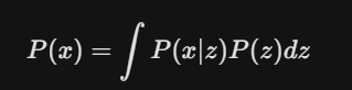
The Training Nightmare: Because z is continuous, there are infinite decimal points to check. To calculate P(x) exactly, the computer would have to run the Decoder for infinite points. This is what we call Intractable — it is a calculation that can never be finished.

3. The Solution: The ELBO Method

Since we cannot solve the Infinite Integral, we take a shortcut called the Evidence Lower Bound (ELBO).

Instead of trying to find that impossible “Total Score,” we calculate a simpler version called ELBO. It’s a mathematical formula that acts as a very good estimate. It allows the computer to train using just a few samples from the Encoder rather than checking the whole infinite space. It turns a forever task into a right now task. In simple terms, it is the sum of two losses:

Total Loss = Reconstruction Loss + KL Divergence

4. The Training Goal: The Two-Part Loss Function

To get the model to learn, we give it a To-Do List with two main tasks. These two tasks make up the Loss Function.

Task A: The Reconstruction Task
The model takes a sample from the latent space and tries to redraw the original image.

Why? This ensures the Decoder knows how to turn abstract numbers into real-looking pixels. If the output looks like the input, the Reconstruction Loss is low.

Task B: The Organization Task (KL Divergence)
This task forces the Encoder to be organized. It tells the Encoder: “Don’t just put codes anywhere. Keep them all close to the center (0) and make sure they have a bit of spread (1).”

Why? This ensures there are no empty gaps in our latent space. By forcing the “clouds” of data to stay close and overlap, the model learns the relationship between different images.

Understanding Reconstruction Loss:

You can think of Reconstruction Loss as a pixel-by-pixel comparison between an original photo and its photocopy.

When we feed a 28 x 28 image into the Encoder, it compresses it into a small code z. The Decoder then tries to “repaint” the 28 x 28 image from that code. Reconstruction Loss tells us exactly how different the Decoder’s painting is from the original.

1. How it works: Pixel-by-Pixel Comparison

Imagine the original pixel value is X and the pixel value generated by the Decoder is X̂.

.The Reconstruction Loss visits every single pixel and asks: “What was the original value, and what did you create?”

2. Two Main Ways to Calculate Loss

Depending on the type of data, we use different mathematical formulas:

Binary Cross-Entropy (BCE): Used for MNIST-style images (mostly black and white, values between 0 and 1). It measures the “probability” of a pixel being white.
Mean Squared Error (MSE): Used for colored or complex images where pixel values vary greatly.
MSE = (X — X̂)²
It calculates the square of the distance between the original and the generated pixel. The bigger the mistake, the larger the loss.

3. How it forces the model to learn Features

If the Reconstruction Loss is high, it means the Decoder painted a “9” that looks like garbage. The Decoder complains: “The 10–12 numbers (z) provided by the Encoder weren’t good enough!”

Through Backpropagation, the Encoder gets penalized. It realizes it must send better instructions (Features) — like the roundness of the 9 or the slant of the 7 — so the Decoder can place the pixels correctly and reduce the loss.

Understanding KL Divergence: The “Librarian” of Latent Space

If we only had Reconstruction Loss, the model would become a memorization machine. It would prioritize accuracy above all else, leading to a catastrophic failure in how it organizes its knowledge.

1. The Problem: The Garbage Gaps

Imagine training the model without KL Divergence. The Encoder wants to make the Decoder’s job as easy as possible. To avoid any confusion between a “7” and an “8,” the Encoder will assign them sets of values (z) that are incredibly far apart:

For a “7”, it might assign the set of values z = [1000, 1000].
For an “8”, it might assign the set of values z = [-1000, -1000].

By scattering these sets of values so far apart, the model creates huge amounts of empty space in between.

Why is this “Garbage”? The Decoder only learns to draw when it sees those specific, far-away values. If you try to generate a new image by picking a random set of values in the middle (like z = [0, 0]), the Decoder has no idea what to do. It has never seen anything in that region during training. As a result, it will just output meaningless garbage or noise. The Latent Space becomes a “broken map” where only a few tiny islands of data exist in a vast ocean of nothingness.

2. The Solution: How KL Divergence Fixes the Map

KL Divergence is the rule that forces the model to be organized. It acts as a mathematical ruler that measures the distance between two probability distributions:

The Encoder’s Guess q(z|x) : The specific mean and variance generated for an image.
The Standard Map p(z): A “Standard Normal Distribution” where the Mean is 0 and the Variance is 1.

KL Divergence tells the Encoder: “You are not allowed to hide your set of values z in the millions or billions. You must pull them all back toward the center (0) and keep them in a tight, overlapping group.”

3. Closing the Gaps: Making the Space “Continuous”

By forcing all sets of values z to stay near the center and maintain a certain spread (Variance = 1), KL Divergence ensures two things:

No Empty Space: There are no “dead zones.” Every part of the map near the center is filled with some information.
Smooth Transitions: Because the sets of values are forced to be close together, their probability clouds naturally overlap.

This overlap is the secret to AI creativity. If you pick a set of values exactly between the “7” cloud and the “1” cloud, the Decoder now understands how to blend them. Instead of garbage, you get a realistic result — like a “slanted 7” or a “curved 1.”

4. Summary: The Tug-of-War

Training a VAE is a constant balance between two competing goals:

Reconstruction Loss wants to push the sets of values z apart to make them distinct and accurate.
KL Divergence wants to pull those sets of values z together to keep the map compact and eliminate the “garbage gaps.”

This “tension” is what makes the model generative. The model is forced to find the most efficient way to describe the “essence” of a 9 while staying within the organized boundaries of the center map.

Part 5: The Backpropagation Miracle — The Reparameterization Trick

We have the architecture and we have the Loss Function. But there is one massive technical roadblock that almost made VAEs impossible to train. It’s known as the “Sampling Problem.”

1. The Problem: The Broken Gradient

To learn, a Neural Network uses a process called Backpropagation. It calculates an error at the end (the Loss) and sends a signal backward through the network to tell each neuron how to adjust its weights.

However, in a VAE, the Encoder produces a Mean and a Variance, and then we sample a set of values z from that distribution.

The Issue: Sampling is a random act. It’s like rolling a die.
The Math: You cannot take a derivative (calculate a gradient) of a random process. If the error signal tries to travel back from the Decoder to the Encoder, it hits the “Sampling” block and stops. The network has no way of knowing how to adjust mean and variance because the path is broken by randomness.

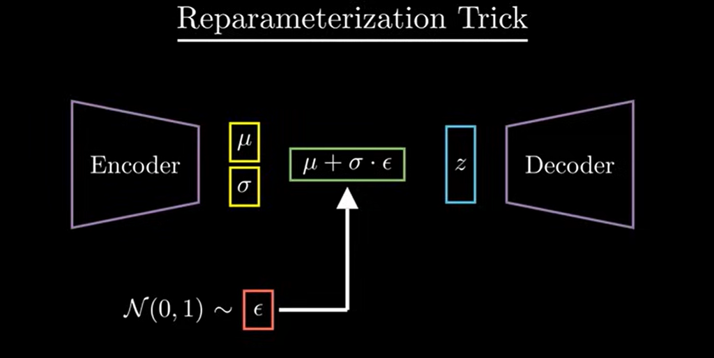
2. The Solution: Moving the Randomness

To fix this, we use a clever mathematical hack called the Reparameterization Trick. We find a way to get a random sample without making the whole process un-trainable.

Instead of letting the Encoder be random, we make it deterministic (predictable) and move the randomness to a separate, independent variable called ε (Epsilon).

We calculate our set of values (z) using this simple equation:

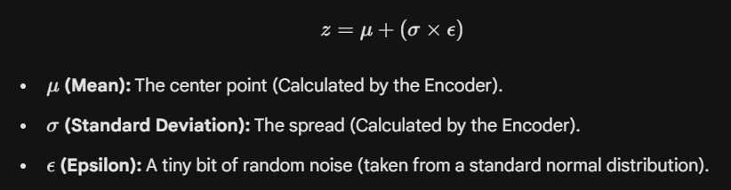
3. Why we need ε ?

You might wonder: “Why not just use z = μ + σ directly?”

If we removed ε, every time the model saw a ‘7’, it would get the exact same z. The randomness would disappear, the “cloud” would shrink into a single point, and our VAE would turn back into a rigid, non-creative Autoencoder.

The Role of ε (For Creativity) :
It acts as a random multiplier. It decides where we land inside the cloud. This forces the Decoder to be “sturdy” and learn all variations of a ‘7’.

4. Why is this a “Trick”?

By writing the equation this way, we have separated the Information from the Noise:

The Information: Mean and variance are now just regular numbers in a math equation. They are not random.
The Noise: All the randomness is trapped inside ε.

The Result: During training, the error signal (gradient) can now flow freely through the plus and multiply signs, back into the mean and variance of the Encoder. The “Randomness” ε just sits on the side like a passenger, not blocking the road.

Code Example for Variational AutoEncoders :

import torch
import torch.nn as nn
import torch.optim as optim
from torchvision import datasets, transforms
from torch.utils.data import DataLoader
import matplotlib.pyplot as plt

device=torch.device("cuda" if torch.cuda.is_available() else "cpu")

BATCH_SIZE=128

data_transform=transforms.Compose([transforms.ToTensor()])
train_dataset=datasets.MNIST(root='./data',train=True,download=True,transform=data_transform)
train_loader=DataLoader(train_dataset,batch_size=BATCH_SIZE,shuffle=True)

# coding the VAE class

latent_dim=64

class VAE(nn.Module):
    def __init__(self,input_dim=784,hidden_dim=256,latent_dim=latent_dim):
      super().__init__()

      # Encoder

      self.fc1=nn.Linear(input_dim,hidden_dim)
      self.fc_mu=nn.Linear(hidden_dim,latent_dim)
      self.fc_log_var=nn.Linear(hidden_dim,latent_dim)

      # Decoder
      self.fc2=nn.Linear(latent_dim,hidden_dim)
      self.fc3=nn.Linear(hidden_dim,input_dim)
      self.relu=nn.ReLU()
      self.sigmoid=nn.Sigmoid()

    def encode(self,x):
      o=self.relu(self.fc1(x))
      return self.fc_mu(o),self.fc_log_var(o)

    def reparameterize(self,mu,log_var):
      std=torch.exp(0.5*log_var)
      eps=torch.randn_like(std)
      return mu+eps*std

    def decode(self,x):
      d=self.relu(self.fc2(x))
      return self.sigmoid(self.fc3(d))

    def forward(self,x):
      mu,log_var=self.encode(x)
      z=self.reparameterize(mu,log_var)
      x_reconstructed = self.decode(z)
      return x_reconstructed,mu,log_var

# coding the loss

def vae_loss(x,x_reconstructed,mu,log_var):
  reconstruction_loss=nn.functional.mse_loss(x_reconstructed,x)
  kl_divergence=0.5*torch.sum(mu.pow(2)+ log_var.exp() - log_var -1)
  return reconstruction_loss+kl_divergence

model=VAE().to(device)
optimizer=optim.Adam(model.parameters(),lr=1e-3)

epochs=5

model.train()

for epoch in range(epochs):
  total_loss=0
  for x,_ in train_loader:
    x=x.view(-1,784).to(device)
    optimizer.zero_grad()
    x_reconstructed,mu,log_var=model(x)
    loss=vae_loss(x,x_reconstructed,mu,log_var)

    loss.backward()
    optimizer.step()

    total_loss+=loss.item()
  avg_loss=total_loss/len(train_loader.dataset)
  print(f"Epoch {epoch+1}/{epochs}, Loss: {avg_loss:.4f}")

# Evaluation

model.eval()

with torch.no_grad():
  x, _= next(iter(train_loader))
  x=x.view(-1,784).to(device)

  x_recon,_,_=model(x)
  x=x.cpu()
  x_recon=x_recon.cpu()

  n=8
  plt.figure(figsize=(12,3))
  for i in range(n):
    plt.subplot(2,n,i+1)
    plt.imshow(x[i].view(28,28).numpy(),cmap='gray')
    plt.axis('off')

    plt.subplot(2,n,i+1+n)
    plt.imshow(x_recon[i].view(28,28).numpy(),cmap='gray')
    plt.axis('off')

  plt.show()

Problems with Variational AutoEncoders :

Although Variational Autoencoders are powerful generative models, they still come with several limitations. VAEs often produce blurry outputs because the decoder learns to model pixel distributions with simple Gaussian assumptions, which struggle to capture sharp details.

Additionally, VAEs lack the ability to generate high-fidelity, photo-realistic images compared to models like GANs, since their likelihood-based training encourages “average-looking” outputs.

Summary :

Variational Autoencoders (VAEs) are powerful generative models that learn a smooth, continuous latent space and can generate new data by sampling from a learned probability distribution. They provide meaningful latent representations, allow smooth interpolation between data points, and create a structured latent space through the combination of reconstruction loss and KL divergence. VAEs are widely used for representation learning, anomaly detection, data compression, and tasks where interpretability of latent factors is important.

References:

Variational Autoencoders in simple language was originally published in Towards AI on Medium, where people are continuing the conversation by highlighting and responding to this story.

Like 0

Liked Liked