To ReLU, or not to ReLU: A Practitioner’s Guide to Solve the “Zombie Neuron” Problem in Deep…

To ReLU, or not to ReLU: A Practitioner’s Guide to Solve the “Zombie Neuron” Problem in Deep Networks

In our brains, neurons constantly filter huge amounts of sensory data, recognizing patterns and ignoring unnecessary information. This is exactly what artificial neural networks do, and it is accomplished through activation functions.

Without activation functions, regardless of how many layers we stack into our neural networks, they will still be useless, as they will simply be a linear combination of their inputs. Activation functions provide the non-linearity needed to learn complex patterns, which is necessary for complex tasks like image recognition, language processing, etc.

The current de facto standard has been ReLU (Rectified Linear Unit) for quite some time now. This is because it has been proven to converge much faster than previous functions, such as Sigmoid and Tanh, and it completely solves the infamous vanishing gradient problem for large inputs (either positive or negative).

But, as we will see, it has a dark side, a mathematical Achilles’ heel that can render our models useless.

The Problem

To understand why a network dies, we must look at the math behind standard ReLU:

ReLU ensures sparsity by retaining only positive activations; it returns 0 for any negative input.¹ While this sparsity improves computational efficiency… however, the negative side of the graph also reveals a major weakness: the value of the gradient is zero.

During the training phase, if the weight update or the bias is extremely negative, the neuron may end up always outputting 0 for any possible input. If the gradient is zero, the neuron’s weights and biases will cease to learn. They will remain stuck in that position for the rest of the hidden layers.

The neuron will never learn again; it will never “wake up”. If the majority of our network is in this position, our network’s power is significantly reduced, resulting in a “zombie network”.

The Symptoms

How do you know that your network is infested with dead neurons? Unlike the exploding gradients, where the NaN errors make it very evident, dead ReLUs will only quietly fail to perform. Here is the list of things to check for:

• Early Training Plateaus: The loss is decreasing at first, but then it plateaus at an unexpectedly early stage, while the accuracy remains low throughout the validation set.
• Extreme Sparsity: While the ReLU network is supposed to have a certain percentage of zero-producing (inactive) neurons (computational efficiency), the activation statistics of our hidden neurons will show that 60% to 80% of the neurons are producing zeros in a “dead neuron” problem.

The Cure

If standard ReLU is killing our network, it is time to upgrade our activation functions. Several robust activation functions have been developed by researchers, which are capable of keeping the gradients flowing:

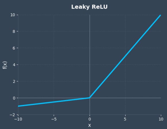
• Leaky ReLU: It is the easiest and most common solution. Instead of a flat zero, Leaky ReLU introduces a small, non-zero gradient (typically a slope of α = 0.01) for negative inputs. It prevents the death of neurons and keep the backpropagation continued by “leaking” a fraction of the input through.²

• Parametric ReLU (PReLU): A further advancement of Leaky ReLU, PReLU does not fix the slope treats the slope α to a non-zero value; instead, it treats it as a learnable parameter.³ In other words, the network learns the best possible value of the slope α.
• Exponential Linear Unit (ELU): Taking it even further, ELU doesn’t just give a straight line as the activation curve for negative inputs. Instead, ELU introduces a gradual, smooth exponential decay curve.⁴ In mathematical terms, the activation function is designed in a way that drastically reduces the chance of a dead neuron.

• Swish & GELU (The Modern Heavyweights): For deep and complex architectures, functions such as Swish (a smooth non-monotonic function with small negative values⁵) greatly improve gradient flow and reduce the dying ReLU problem. GELU (Gaussian Error Linear Unit) weights the inputs by their percentiles and is currently the standard for transformer architectures such as BERT and GPT.⁶

The Benchmark (Visualizing the Zombie Network)

We will see the catastrophic impact of the dying ReLU problem, in practice. We set up a controlled benchmarking experiment using PyTorch.

The Experimental Setup

We designed a “stress test” for our activation functions by training two identical neural networks on the Fashion-MNIST dataset (a standard image classification task with 10 classes).

Here are the specifications of our architecture:

• Network Type: A standard Feed-Forward Neural Network (Multi-Layer Perceptron).
• Layers: An input layer (flattening the 28×28 images into 784 features), followed by two hidden layers with 256 neurons each, and a final output layer of 10 neurons.
• Optimizer: Adam optimizer with a learning rate of 0.001.
• Training Duration: 30 epochs.

The Catch (The Sabotage)

To intentionally trigger the “dead ReLU” phenomenon, we handicapped both networks by initializing the biases of the hidden layers to a constant negative value (-1.0). While in a well-initialized network, neurons die off slowly over time due to large negative weight updates, here we forcefully push the pre-activation values into the negative domain right from Epoch 1 by starting with negative biases. This will simulate a worst-case training scenario.

We then equipped Network A with the standard ReLU function and Network B with the Leaky ReLU function (α = 0.01) to see who would survive.

import torch
import torch.nn as nn
import torch.optim as optim
import torchvision
import torchvision.transforms as transforms
import matplotlib.pyplot as plt
import numpy as np

# Neural Network Architecture
class BenchmarkNetwork(nn.Module):
    def __init__(self, activation_function):
        super(BenchmarkNetwork, self).__init__()
        self.flatten = nn.Flatten()
        # A 3-layer Multi-Layer Perceptron (MLP)
        self.fc1 = nn.Linear(28 * 28, 256)
        self.fc2 = nn.Linear(256, 256)
        self.fc3 = nn.Linear(256, 10)
        self.activation = activation_function
        
        # Intentionalnegative biases to encourage "Zombie Neurons"
        nn.init.constant_(self.fc1.bias, -1.0)
        nn.init.constant_(self.fc2.bias, -1.0)

    def forward(self, x):
        x = self.flatten(x)
        
        x = self.fc1(x)
        a1 = self.activation(x)
        x = self.fc2(a1)
        a2 = self.activation(x)
        out = self.fc3(a2)
        return out, a1, a2 # Returning activations for our histogram

def train_and_track(model, train_loader, epochs=30):
    criterion = nn.CrossEntropyLoss()
    optimizer = optim.Adam(model.parameters(), lr=0.001)
    
    loss_history = []
    final_activations = []

    model.train()
    for epoch in range(epochs):
        epoch_loss = 0
        for images, labels in train_loader:
            optimizer.zero_grad()
            outputs, a1, a2 = model(images)
            loss = criterion(outputs, labels)
            loss.backward()
            optimizer.step()
            epoch_loss += loss.item()
            
        loss_history.append(epoch_loss / len(train_loader))
        
    final_activations = torch.cat([a1.view(-1), a2.view(-1)]).detach().numpy()
    return loss_history, final_activations

# Fashion-MNIST data
transform = transforms.Compose([transforms.ToTensor(), transforms.Normalize((0.5,), (0.5,))])
trainset = torchvision.datasets.FashionMNIST(root='./data', train=True, download=True, transform=transform)
train_loader = torch.utils.data.DataLoader(trainset, batch_size=64, shuffle=True)

# Run the ReLU model
relu_model = BenchmarkNetwork(nn.ReLU())
relu_loss, relu_acts = train_and_track(relu_model, train_loader)

# Leaky ReLU with a slope of 0.01 for negative inputs
leaky_model = BenchmarkNetwork(nn.LeakyReLU(negative_slope=0.01)) 
leaky_loss, leaky_acts = train_and_track(leaky_model, train_loader)

Analyzing the Results

The results of this 30-epoch benchmark are striking. When we plot the training loss and the distribution of the final layer activations, the difference between a functional network and a “zombie” network becomes clearly visible.

1. The Training Loss (Left Plot)

• The Standard ReLU (Red Line): The red line completely flatlines at a high loss value (above 2.0) from the very first epoch. Since we handicapped the network with negative bias, it is not learning anything. The negative bias forced the inputs below zero, the standard ReLU function outputted 0 post-activation, resulting in a gradient of 0 during backpropagation. The optimizer cannot update the weights, leaving the network permanently stuck without learning anything at all.
• The Leaky ReLU (Green Line): The green line tells a different story of recovery. Despite starting with the exact same handicap (negative biases), Leaky ReLU’s small negative slope (α = 0.01) allows a tiny, non-zero gradient to flow backward through the network. This “leak” is just enough for the optimizer to adjust the weights, pull the pre-activations back into the positive domain, and drive the loss down over 30 epochs.

2. Distribution of Hidden Layer Activations (Right Plot)

This histogram, plotted on a logarithmic scale, shows us the ground truth for our hidden layers.

• The Zombie State (Red): The terrifying statistic: 99.2% Dead. Almost every single neuron in the standard ReLU network is outputting exactly 0.0. The network’s capacity has been mathematically obliterated.
• The Healthy State (Green): The Leaky ReLU network shows a rich, wide distribution of activation values stretching from 0 up to 35. The neurons are actively firing, processing the complex patterns of the Fashion-MNIST dataset, and contributing to the model’s predictive power.

Conclusion

While standard ReLU is computationally efficient and perfectly adequate for many standard tasks, it operates without a safety net. If our gradients explode or our initialization is slightly off, a massive percentage of our network can silently die. By simply switching to a variant like Leaky ReLU, PReLU, or ELU, we can provide our model with a crucial escape route from the zero-gradient trap, ensuring a much more robust and stable training process.

References

¹ Nair, V., & Hinton, G. E. (2010). Rectified linear units improve restricted Boltzmann machines. In Proceedings of the International Conference on Machine Learning (ICML) (pp. 807–814). https://www.cs.toronto.edu/~hinton/absps/reluICML.pdf

² Maas, A. L., Hannun, A. Y., & Ng, A. Y. (2013). Rectifier nonlinearities improve neural network acoustic models. Proc. ICML, 30(1).

³ He, K., Zhang, X., Ren, S., & Sun, J. (2015). Delving deep into rectifiers: Surpassing human-level performance on ImageNet classification. In Proceedings of the IEEE International Conference on Computer Vision (ICCV) (pp. 1026–1034).

⁴ Clevert, D.-A., Unterthiner, T., & Hochreiter, S. (2015). Fast and accurate deep network learning by exponential linear units (ELUs). arXiv. https://arxiv.org/abs/1511.07289

⁵ Ramachandran, P., Zoph, B., & Le, Q. V. (2017). Searching for activation functions. arXiv. https://arxiv.org/abs/1710.05941

⁶ Hendrycks, D., & Gimpel, K. (2016). Gaussian error linear units (GELUs). arXiv. https://arxiv.org/abs/1606.08415

---

To ReLU, or not to ReLU: A Practitioner’s Guide to Solve the “Zombie Neuron” Problem in Deep… was originally published in Towards AI on Medium, where people are continuing the conversation by highlighting and responding to this story.