The Problem Chain That Led to Transformers
Word embeddings, attention, and positional encodings and the specific problem each one was built to solve.
Blogging my understanding as I go through the lecture series of “CS 639: Introduction to Foundation Models” at University of Wisconsin-Madison.

How Do Machines Even Understand Words?
Before we get into the fancy stuff, it’s worth pausing on this simple question. Text is just characters to a machine, so how do we get it to understand meaning?
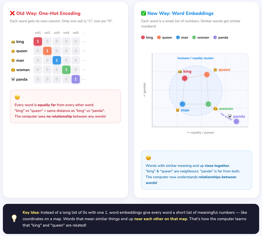
A few naive solutions come to mind: Assign each word a unique integer ID (integer encoding). Integer IDs simply imply an ordering (“cat” = 3, “dog” = 4… so dogs are somehow more than cats here).
Or use one-hot vectors, they are sparse, high-dimensional and carry zero semantic information, i.e., “king” and “queen” are just as “far apart” as “king” and “panda”, even though intuitively one pair is far more related than the other. Both these methods lacked something.
The ideal solution is something richer: A dense, low-dimensional vector where similar words end up close together in space. So “king” and “queen” are neighbors. This is the core idea behind word embeddings.
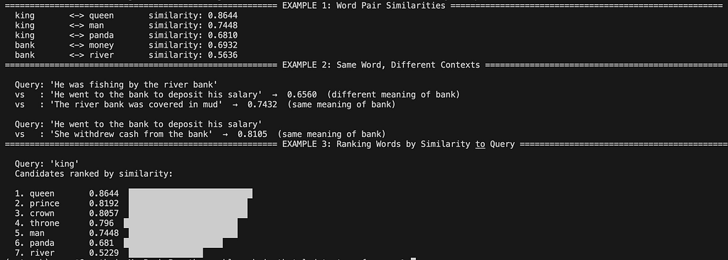
To see this concretely, look at the BERT cosine similarity scores between word pairs in the image below.
- “king” and “queen” score 0.86 -> they’re close neighbors in embedding space.
- “king” and “panda” score 0.68 -> much further apart, as we’d expect.
- “bank” (more interesting case): its similarity score with “money” versus “river” differs depending on the sentence it appears in. That’s because BERT is a contextual model, the embedding of “bank” shifts based on surrounding words unlike static embeddings. (We’ll see how this works when we get to attention.)
However, static models like Word2Vec or GloVe don’t do this; “bank” always maps to the same vector, regardless of whether you’re at a river or an ATM.
But even good word embeddings leave a deeper problem unsolved. With static embeddings, each word is assigned a vector independently of context. In models like Word2Vec or GloVe, “bank” in “river bank” and “bank” in “reserve bank” still produce identical representations, there’s no mechanism for words to influence one another.
We’ve represented words, but we haven’t represented language. To do that, we need a model that processes words as a sequence, allowing context to flow between them.
Before Attention: The RNN Era
RNNs process sequences step by step, maintaining a hidden state that carries forward information from the past.
The diagram below captures the core idea, blue nodes are states, yellow nodes are inputs. Each state receives the current input x(t) and the previous state s(t-1), then produces a new state and an output. The temporal connection flows strictly left to right.
Classical RNNs
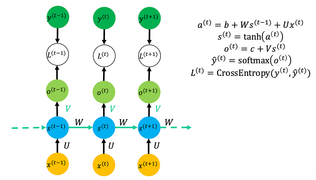
At each time step, the update looks like this: 𝑎(𝑡) = 𝑏 + 𝑊 . 𝑠(𝑡−1) + 𝑈 . 𝑥(𝑡)
Unlike a fully connected network which processes everything at once, an RNN shares the same weights across all time steps.
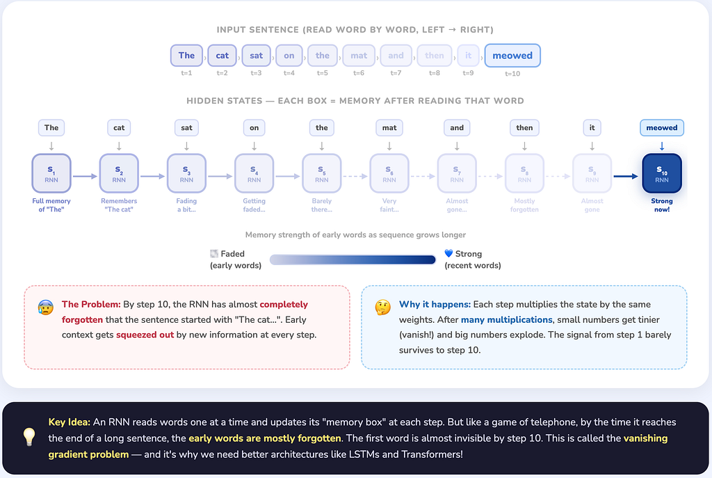
The big idea: we don’t need to change the weights as we move through the sequence. The temporal connection flows left to right, and the hidden state in theory keeps track of past context.
In practice though? Long sequences break this. By the time we’re 50 tokens in, the state s(t) has been squished through so many non-linearities that early context is essentially gone. We could make the state bigger, but that’s just slapping a larger band-aid on the same wound.
LSTMs and GRUs to the Rescue (Sort Of)
- Both were designed to address the vanishing memory problem in vanilla RNNs

- The key upgrade in LSTMs is a separate cell state, a kind of long-term memory lane that runs alongside the hidden state. Gates decide what gets written to it, what gets read from it and what gets erased. GRUs simplify this with fewer gates but achieve similar results with less compute.
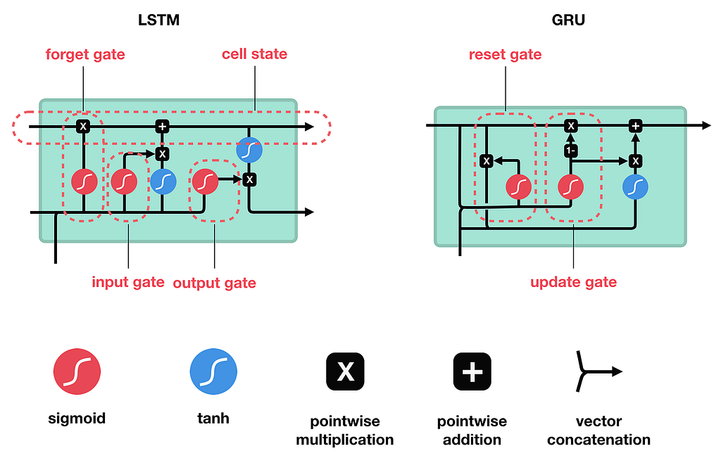

Both helped a lot. But zoom out and the fundamental bottleneck remains: no matter how smart the gating, the entire history of the sequence still has to be squeezed into a fixed-size vector before being handed to the next stage.
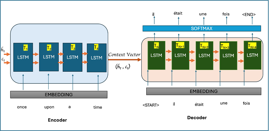
Notice how everything, the entire input sentence gets compressed into one context vector before the decoder ever sees it. That single vector is the bottleneck.
For short sentences this is fine.
For long documents, paragraphs, or books, we’re asking one vector to remember everything.
Something always gets lost.
That is the problem attention was built to solve.
Attention
The insight that changed everything: Instead of summarising the past into a single vector, what if every word could directly look at every other word and decide how much to pay attention to it?
This is self-attention.
Take the classic example, the word “bank”. In isolation, it’s ambiguous. But in context:
- “He was fishing by the river bank” — — > A geographical feature
- “He went to the bank to deposit his salary” — — > A financial institution

With self-attention, when encoding “bank,” the model computes a score between “bank” and every other word in the sentence. “River” gets a high score in the first sentence, “deposit” and “salary” get high scores in the second. The resulting representation of “bank” is a weighted blend of all other word representations and that blend carries the context.
How it works mathematically (QKV)
Each input token gets projected into three vectors: a Query (Q), a Key (K), and a Value (V), via learned linear transformations.

The attention scores are then computed as:
Attention(Q, K, V) = softmax(QKᵀ / √d_k) · V
Intuitively, QKV works like this:
- Query is what the current token is looking for
- Keys are what every other token offers
- Values are the information that gets passed forward
The dot product QKᵀ measures how good a match they are. Dividing by √d_k keeps the scores from getting too large before the softmax. The softmax turns the scores into weights, and those weights are applied to the Values to produce the final output, a context-aware representation of each token.

Mathematically, this involves a lot of dot products and matrix multiplications. However, all the output vectors z1, z2, z3… are independent of each other and can be computed in parallel. This is the foundation of multi-head attention, run several attention computations in parallel, each potentially learning to focus on different kinds of relationships (syntax, co-reference, semantics), then concatenate and project the results.

To understand more in detail, check out https://jalammar.github.io/illustrated-transformer/.
The Problem Attention Introduced: Order Blindness
Self-attention is powerful, but it has a glaring issue, it treats the input as a set, not a sequence. Shuffle the words in a sentence and attention produces the same representations. Word order is entirely invisible to it.

This matters enormously. “The dog bit the man” and “The man bit the dog” contain the same words, same attention scores between each pair, but completely different meanings.
Positional Encodings
The fix is to inject some notion of position into the embeddings before feeding them into the attention layers.
Integer Encoding: The Naive Approach
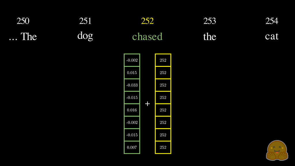
The simplest idea: just add the word’s index to its embedding vector — w1 + 1, w2 + 2, and so on. This works in principle but breaks in practice. For long sequences, the positional values grow large and completely dominate the embedding values, distorting the semantic information the embeddings were trained to carry.
Binary Encoding: A Better Attempt
So, what if instead of raw integers, we encode position in binary? Every position gets a fixed-length binary vector — position 0 is [0, 0, 0, 0], position 1 is [0, 0, 0, 1], position 2 is [0, 0, 1, 0], position 7 is [0, 1, 1, 1], and so on.
This is already much better than raw integers — the values are bounded (always 0 or 1), the representation is unique per position, and the pattern has a nice structure where different bit positions toggle at different frequencies. The least significant bit flips every step, the next bit every two steps, the next every four, and so on.

But, binary encoding still has a problem: The values are discrete, only 0s and 1s. Discrete jumps are hard for neural networks to interpolate between. A network that has seen position 4 ([0,1,0,0]) and position 5 ([0,1,0,1]) has no smooth signal to generalise from. There’s also a representational ceiling, with d bits we can only encode 2^d positions, which becomes a hard limit.

What we really want is the spirit of binary encoding, different frequencies toggling at different rates, bounded values, unique per position, but in a continuous, smooth form that a neural network can work with gracefully.
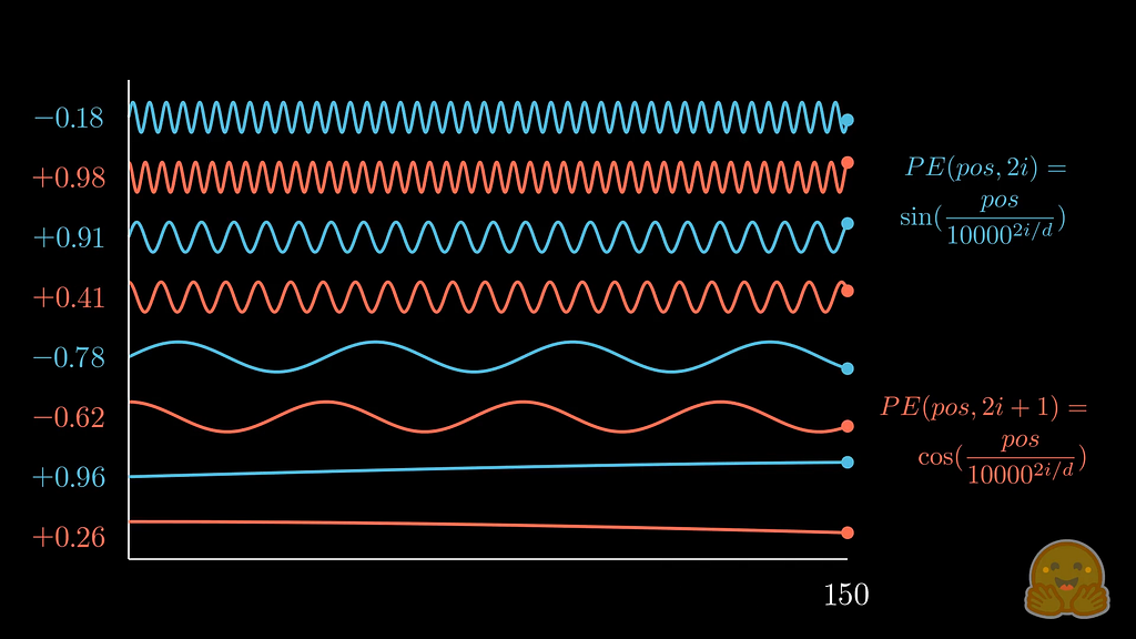
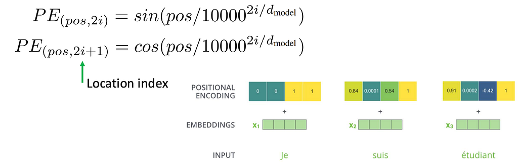
Sinusoidal Encoding: Continuous Binary
This is exactly what the sinusoidal encoding from Attention Is All You Need (Vaswani et al., 2017) gives us. Intuition maps directly onto binary: the higher-indexed dimensions use very low frequencies (slow oscillation, like the most significant bit), and the lower-indexed dimensions use high frequencies (fast oscillation, like the least significant bit). Every position gets a unique combination of values across all dimensions: A continuous fingerprint.
Instead of discrete bit toggles, use sine and cosine waves at different frequencies:
Why does this work?
- The values are always bounded between -1 and 1, so they never overwhelm the embeddings
- Each position gets a unique encoding
- The relative distance between positions is consistent, the model can generalise to sequence lengths it hasn’t seen during training
- It’s fixed, no learned parameters needed (though learned positional encodings are also used in practice)
Sinusoidal encoding is fixed and elegant, but it has a subtle limitation, position is baked into the token before attention ever runs. By the time the model computes Q·Kᵀ, the positional signal has already been mixed into the embedding and can’t be cleanly separated from the semantic content.
RoPE and ALiBi
RoPE (Rotary Position Embeddings) takes a different approach. Instead of adding position to the embedding upfront, it encodes relative position inside the attention operation itself, by rotating the Query and Key vectors by an angle proportional to their position before the dot product. The result is that attention scores naturally reflect how far apart two tokens are, not just what they contain. Absolute position drops out; relative distance is what remains.
This turns out to matter enormously at scale. A model trained on sequences of length 2048 with sinusoidal encodings struggles when we hand it a 8192-token document at inference, the positional patterns it saw during training simply don’t extend cleanly. RoPE generalises more gracefully, which is why it has become the default in virtually every production LLM built in the last two years, LLaMA, Mistral, Qwen, and most of their derivatives all use it.
ALiBi takes a different angle entirely, rather than encoding position as a vector transformation, it applies a linear penalty directly to attention scores based on distance. No positional vectors at all; just “the further away, the less attention.” Simpler, but surprisingly effective for long-context generalisation.
The sinusoidal version remains the conceptual foundation worth understanding first, RoPE and ALiBi both make more sense once we’ve seen what problem they’re improving on.
Putting It All Together

The full pipeline in a transformer looks roughly like this:
- Tokenise the input text into tokens
- Embed each token into a dense vector (word embedding)
- Add positional encodings so the model knows where each token sits
- Pass through multi-head self-attention layers, where each token attends to all others
- Feed through feed-forward layers, repeat N times
- Produce output
Each component solves a specific, well-motivated problem.
Words need meaning → Embeddings. Embeddings are context-blind → RNNs. RNNs forget → LSTMs/GRUs. LSTMs hit a bottleneck → Attention. Attention is order-blind → Positional encodings.
None of them are magic in isolation; the magic is how cleanly they compose.
Further Reading/References:
- Vaswani et al., Attention Is All You Need, 2017
- Jay Alammar — The Illustrated Transformer
- Designing Positional Encodings — Hugging Face
- RNN vs LSTM vs GRU vs Transformers — GeeksforGeeks
Credits:
- Figures 1, 4, 9, 13: Generated using Claude Sonnet 4.5 for illustration
- Figure 3, 20: CS639 Slides, UW-Madison
- Figure 5: RNN, LSTM, GRU — LinkedIn
- Figure 6: LSTM vs GRU — AI Stack Exchange
- Figure 8: Encoder-Decoder Architecture — GoPubby
- Remaining figures are taken from the “further reading” links
This is part of an ongoing series as I work through the Introduction to Foundation Models lectures. More to come, hopefully!☺
The Problem Chain That Led to Transformers was originally published in Towards AI on Medium, where people are continuing the conversation by highlighting and responding to this story.