The Journey of Backpropagation in Neural Networks

digitado ⋅ 28 de December de 2020

I’ve always wondered as to what happens in the ‘backend’ of the training process in Neural Networks. The training process is essentially the ‘meat’ of the model; without efficient and effective training the model will not be able to accurately predict/classify or accomplish a task with newly unseen data.

Neural Networks have always been held as a very useful system in prediction analysis, recommendation engines, modeling and a lot more; it is because has the ability to extract complex patterns and relationships between the input and output data. This is because of the numerous layers of neural networks, that make the machine learning ‘deep’.

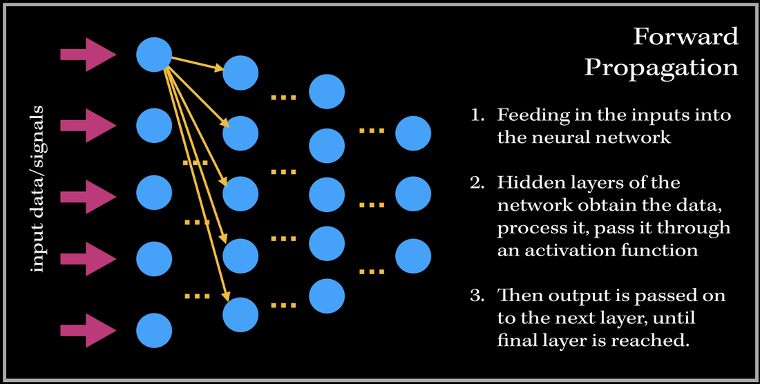
So what does the training process of this neurological-biological computer model-system (aka neural network) look like? It consists of two phases: 1). Forward Propagation and 2). Back propagation. Once we have preprocessed the dataset (such as normalization, reshaping your data to a specific dimension..etc.), we are ready for the training process. We first forward propagate our data—meaning we feed in the inputs into our built neural network.

I like to think of forward propagation consisting of three simple steps: 1) Send in a data point (or a subset of training data points), 2) the layers obtain the data, process it (by computing the dot product), and pass it into some non-linear activation function (ReLU, Sigmoid, Leaky ReLU), 3). Output from previous layer is passed to next layer. The process continues until we have reached the final layer.

Before we get into the deep math, let’s define some variables. These definitions are applied to every example in this blog post!

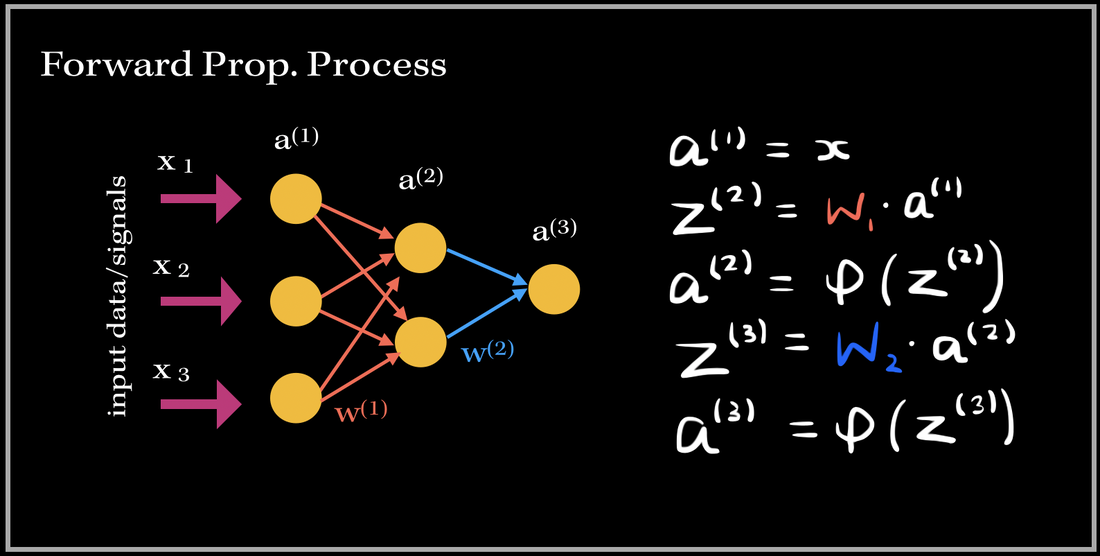
a denotes the neuron value at a particular level of the network (level number is denoted as a superscript of a)
x denotes the input fed into the neural network
w denotes the set of weights at each level
z denotes the dot product of the weights and the previous layer inputs
The activation function is denoted as the sigma symbol. We will be using the sigmoid function for the activation.

SO, what happens after we have passed an instance of our training dataset to the network?

Back Propagation

This is where back propagation comes in. Back-propagation is essentially an algorithm used in training neural networks and is used to improve the model’s performance/accuracy. Our neural network will update its parameters (weights and biases) once every time a number of samples is passed into the network (aka: an epoch in gradient descent algorithm).

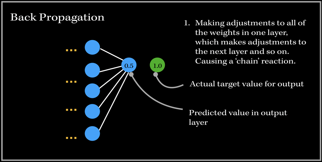
Basically, in Back Propagation, we need to adjust the weight parameters based on our loss function — whether it be calculating the mean squared loss, absolute mean loss or any other loss function we use — and our updated weights must head towards the right direction (in reducing the loss).

Let’s look at an example, and focus on one specific output neuron in a neural network model. We first pass in our input training data, and get a single output neuron of 0.5. However, the specific target value for the neuron is 1.0, so the cost function computes the error, and our optimizer uses the loss to back-propagate and change the weights to minimize the loss. This is why the process is at times called back-propagation of errors, since updates to one layer impact the next layer, and because of this backwards calculation technique, we are preventing redundant calculations.

To do this, we need to figure out how much of an impact does a certain weight (between a node from one layer and a node from the previous layer) have on the cost function. Does the weight have a very low impact (ie. the cost function doesn’t drastically differentiate when the weight parameter changes), or does it have a very important contribution towards minimizing the loss? In order to find this out, we need to look into a very important operation: partial derivatives.

The Process

The back-propagation process starts from the output layer, where the predicted output value is analyzed with the targeted score, using our cost function.
The partial derivative of the cost function with respect to each weight parameter is then computed. This forms the gradient vector — a vector of all the partial derivatives of each weight.
As per the gradient descent algorithm, the weights (parameters) are then modified by subtracting the gradients multiplied by a constant factor (learning rate).

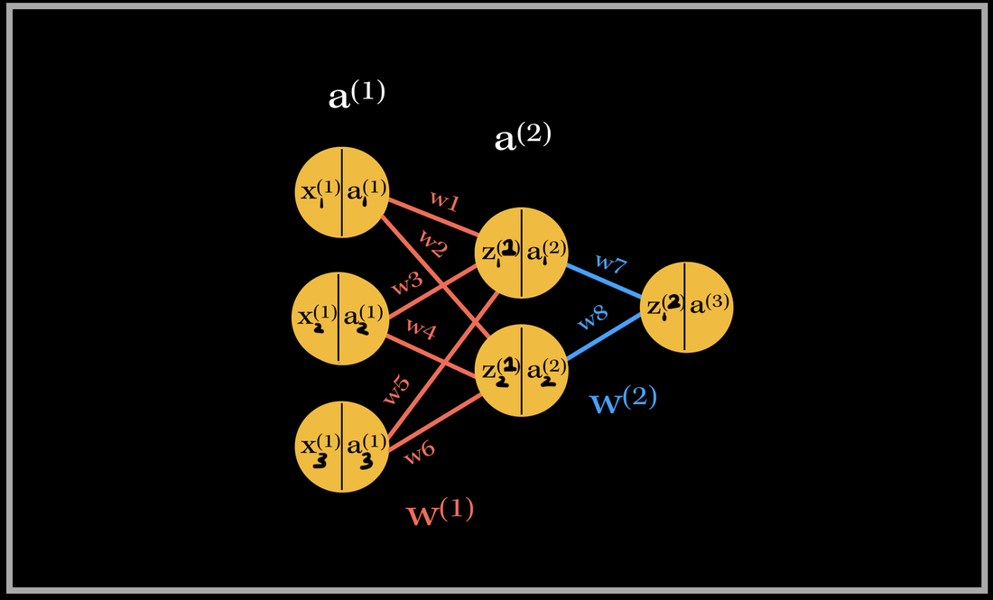
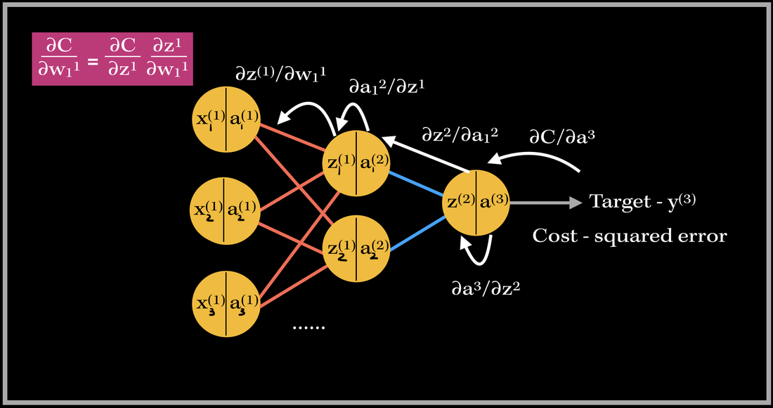
Let’s go do a back propagation run through with an example. Say we had a neural network with 3 input neurons, 2 neurons in the hidden layer, and 1 output neuron.

Neural Network Model with denoted weights, activation values, and dot product values (in neurons)

NOTE: In each neuron, the number on the left side is the input, and number on the right side is the activated input (passed through activation sigmoid).

Back-propagation of the output layer

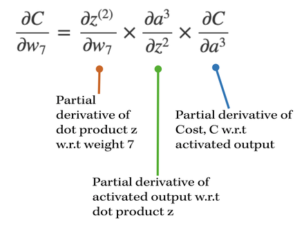
The total number of weights in this network is 8. We have 6 weights in the first layer and 2 weights in the second layer. Let’s first focus on the computing the partial derivative of the cost with respect to one of the weights contributing towards the output neuron: w7. What is the partial derivative of C, the cost, w.r.t to w7, weight 7?

We can express the partial derivative of the cost with respect to weight 7 as the product of 3 partial derivatives by using the Chain Rule.

Essentially, the equation breaks down into three main parts, beginning from a specific derivative and branching out from there.

The activation output, a^(3) is a function of weights in z^(2), and consequently is a function of the weights in w[2] (w7, w8).
Therefore, we can take the derivative of the cost with respect to the output neuron value, a^3, and the utilize the chain rule by branching out and taking the derivative of the output w.r.t to the dot product, z^(2). Finally, in order to express the derivative with respect to the weight 7, we take the derivative of z^(2), the dot product, with respect to weight 7.
By multiplying these three derivatives together, we can basically compute the update for weight 7!

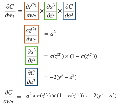
After computing the partial derivatives, we have a final update value for weight 7. Now, the next step is to simply repeat this process for all weights in a recursive way, and update the weight value via gradient descent.

*NOTE: The algorithm substitutes the numerical values into the update equation, in order to perform the gradient descent update for weight 7!*

Back-propagation of a hidden layer

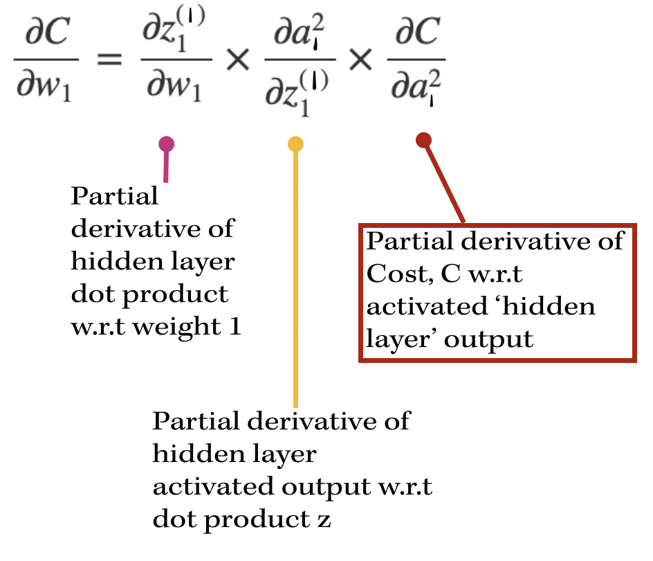
Now, let’s back propagate to the first layer, and compute the gradient of weight 1, w1. The partial derivatives will look slightly different this time, since the cost isn’t directly associated with the hidden layer outputs. With our focus on weight 1, the partial derivative of the cost w.r.t w1 is going to depend on the partial derivative of the cost w.r.t. the output of the hidden layer neuron. This will look like:

While the first two partial derivatives are similar to what we saw in the previous output layer back propagation, the third derivative looks slightly different.

In order to find the update of weight 1, we need to find derivative of the cost function with respect to the hidden layer activated output.

The cost function is indirectly influenced by the activation in the hidden layer. By indirectly influenced, I mean that w7 contributes to the cost function by being multiplied with the hidden layer output.

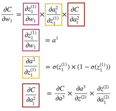
So in order to find the partial derivative with respect to the hidden layer output, we need to include the next layer’s weight’s contribution towards the cost. Therefore, we need to include the weights that are being multiplied by the activation output of the particular hidden layer’s neuron. In this case, it’s only one weight: w7. However, if there are multiple weights contributing, we would have to add them to the equation as well.

So in this case, we can see some similarities and yet some differences. The first derivative in this case evaluates to a^(1), since we are now focusing on the previous layer and set of inputs to the hidden layer (which is a^(1), in the neural network model above).

The next derivative is simply the derivative of our activation, in this case the sigmoid function.

The next derivative is the most interesting part: it is composed of 3 more partial derivatives.

The partial derivative of the Cost w.r.t. the hidden layer activation is broken down again into three parts: 1). First starting from the cost w.r.t to the output activation, then 2). the activation w.r.t the output dot product, 3). then the output dot product w.r.t. hidden layer activation. As you can see there are many terms being repeated in finding the updates for both weights 1 and 7!!

This basically sums up finding the gradient of the network. As you can see, it requires lots of computation and derivatives!! Imagine the workload of computing the gradient vector of bigger neural networks with millions of parameters and neurons–backward propagation does this by using the previous layer’s computations to compute the updates for the next layers! It’s an amazing feat!

Back propagating in action

Back propagation in action for weight 1.

So this is where ‘back propagating the errors’ comes into play. The image above is an example of back propagation in action for weight 1. The previous partial derivatives are reflected in the update value for weight 1. The white arrows show the path of each derivative computation for weight 1’s update.

This same process occurs for every weight in the network during back propagation. Back Prop is one of the most important parts in training supervised learning neural network models! 🙂

Like 0

Liked Liked