
The Geometry of Attention: One Space, Two Operators

How two operators in one space reveal what four projections hide
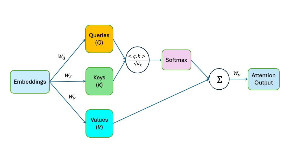
The goal of single-headed attention is to enhance the contextual awareness of a fixed token, or query, based on content from other tokens. This is accomplished in three steps: first, the relevance of one or more tokens to the query is scored; second, the relevance scores are converted into attention weights; and third, the content of scored tokens are combined with the attention weights to arrive at a contextual update to the token of interest.
Explanations of attention emphasize projection matrices for queries (Q), keys (K), and values (V), along with scaled dot products, softmax normalization, and weighted averages. We call this the QKV model of attention.
Attention works remarkably well. But the explanation feels ad hoc. Why four projections? Why multiple spaces? Why this particular sequence of operations?
To better understand attention, we step back from the QKV model and reformulate attention to operate solely in one space.
A simpler formulation of attention
Let E be the high-dimensional vector space that contain all token embeddings and let X be a sequence of token embeddings representing an input prompt. Designate an embedding q ∈X as a query. The problem is: how do we contextually update q based on content from the tokens in X.
We model attention using two transformations:
- A bilinear form, M, that assigns a relevance score to ordered pairs of embeddings
- A linear operator, F, that transforms a token embedding into a content vector of the same size
The two operators play complementary roles: M determines which tokens a query should attend to; F determines what content each token contributes. One space, E, and two operators, M and F — we call this the EMF model of attention.
So, what are these operators?
Relevance as a bilinear form
In the QKV model, relevance between two tokens is computed by projecting one token into query space, the other into key space, and taking a scaled dot product.
In the EMF model relevance between two tokens is computed by the bilinear form, M, defined by:

where W_Q and W_K are query and key projection matrices from the QKV model. The relevance score M(x1, x2) quantifies the degree to which x1 attends to x2, or equivalently, how relevant x2 is to x1.
Relevance scoring in the QKV model can be viewed as a learned “factorization” of M as visualized in the following commutative diagram:
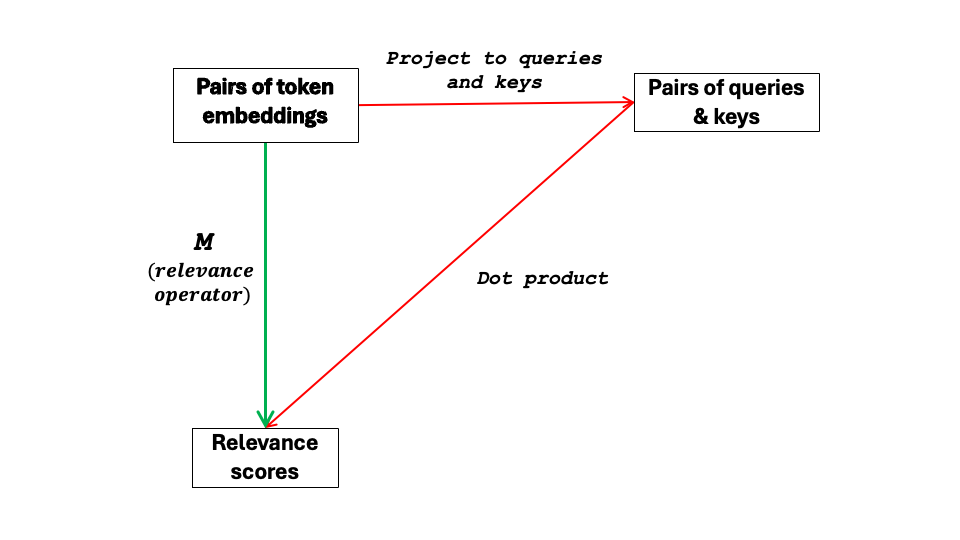
The green path applies M to ordered pairs of embeddings to obtain a relevance score in a single step. The red path factors M by first projecting to an intermediate Q × K product space and then mapping to a scalar value by the dot product. Both paths arrive at the same relevance score, i.e., the diagram commutes.
This equivalence has two consequences. First, the red path, which is implemented in QKV, is not fundamental; it is a computationally efficient factorization of M. Second, taking the green path, we can compute relevance scores in E without queries and keys. Moving relevance scoring over to E reveals its underlying geometry.
The geometry of M
Setting x1 equal to q and letting x2 be any embedding, turns M into the linear functional, M(q, ·), that scores the extent to which q should attend to the embedding. This scoring system stratifies E into parallel hyperplanes of constant relevance — the level sets of M(q, ·) — where relevance scores are determined based on level set membership.
Since M(q, ·) is a linear functional on E, it can be written as an inner product with a single vector — the relevance gradient r_q = (W_Kᵀ W_Q )q. This vector is perpendicular to the level sets of M(q, ·) and points in the direction of increasing relevance. A token’s relevance score is determined entirely by its projection onto r_q; tokens on the same level share the same inner product, hence the same score. Different queries produce different relevance gradients, each orienting the level sets differently and imposing its own directional notion of relevance on E.
The level set geometry of M(q, ·) also stratifies the tokens of the prompt X. The relevance scores that support this stratification are the raw inputs from which attention weights are inferred.
Since every token in X serves as a query, we have a family of linear functionals — one per token — each inducing a different stratification of X by relevance score. Running all the linear functionals in parallel, we obtain a set of relevance scores for all the tokens of X in a single step.
Other geometries related to M constrain the directions in E that participate in relevance scoring — tokens in the right-null space of M are invisible to every query; and as q varies, the relevance gradient to the level sets is confined to a low-dimensional subspace of E. These geometries shape what attention can and cannot see — subject matter for a future article.
Let’s move on to the linear operator F.
Content as a linear operator
Relevance alone does not determine context. Once attention decides which tokens matter, it must decide what information they contribute.
In the QKV model, content is extracted by projecting a token’s embedding into a low-dimensional subspace of values. This implementation works — but it obscures a simpler structure.
In the EMF model, the linear operator F transforms a token’s embedding into a content vector of the same size using

where W_V and W_O are projection matrices from the QKV model and x_i is a token embedding in E.
The following commutative diagram shows how F in the EMF model factors through the value space of the QKV model.

The green path applies F directly to a token embedding to obtain a content vector in E. The red path factors F by first projecting to a lower-dimensional value space and then linearly mapping back to E. Both paths arrive at the same content vector, i.e., the diagram commutes.
Two conclusions: content can be extracted without first projecting to a lower-dimensional value space; and moving content extraction to E reveals its underlying geometry.
The geometry of F
Applying F to the token embeddings of X produces a corresponding sequence of content vectors in E — the raw material from which a query’s contextual update is computed. These content vectors are computed once and shared by all queries of the prompt.
Geometrically, F reshapes token embeddings for content by amplifying certain directions in E, suppressing others, and annihilating the rest. Its singular values determine the hierarchy: large singular values mark directions that F treats as content-rich; directions in F’s null-space are erased entirely. Unlike M, which imposes a different geometry for each query, F defines a single content geometry that applies to all queries.
The range of F is the subspace of E where context takes shape. Every content vector in the EMF model lies in this subspace. Importantly, the weighted average of these context vectors also lies in this subspace. That is, content is aggregated into context in the range of F.
From geometry to inference
Geometry tells us what tokens a query should focus on for content. But it doesn’t tell us how much focus relative to other tokens. That requires inference.
Inference means converting relevance scores to attention weights. This step can be framed as a free-energy minimization problem: find the probability distribution over X that best fits a query’s relevance scores without collapsing all weights onto a single token — a tradeoff enforced by an entropy penalty. The solution turns out to be the softmax, a closed-form mapping from relevance scores to attention weights.
Critically, softmax is not learned. It is a fixed function hardwired into the transformer architecture. What the network actually learns is the bilinear form M, which generates free-energy minimization problems on-the-fly — one for each q ∈ X— that are quickly solved by softmax.
Geometry determines where to look. Inference determines how strongly. Together, they prepare the ground for aggregation of content into context.
From geometry to aggregation
The question now becomes: how do we aggregate the content vectors of F into a single contextual update vector taking into account the attention weights obtained by M?
The answer is the weighted average — but why? At least four different lines of reasoning point to the same answer.
From least squares: the weighted average is the unique point in E that minimizes the weighted sum of squared distances to the content vectors. M determines the weights; F determines what gets weighted.
From geometry: the weighted average is the barycenter — the center of mass of the content vectors under the attention weights. It is the unique point where the weighted displacements from the content vectors cancel.
From probability: treating attention weights as a probability distribution over content vectors, the weighted average is the expected value — the summary that minimizes expected squared distance to the content vectors.
From linearity: the weighted average is the only aggregation rule that is both linear in the content vectors and faithful to the weights — meaning each weight is respected proportionally, so that concentrating all weight on a single token recovers that token’s content vector exactly.
Least squares, geometry, probability, and linearity each point to the weighted average as the way to aggregate content into context for a given distribution of attention weights.
Why it matters
The EMF model for single-headed attention does more than reformulate attention — it reveals geometric structure that the QKV model obscures, with consequences for both understanding and engineering.
The most immediate consequence is that structural constraints become readable. M’s null space identifies directions in E that are invisible to every query — tokens aligned with these directions cannot influence relevance scoring regardless of context. F’s null space identifies content that is erased entirely, while its range defines the subspace where all contextual updates must live. These are hard constraints on what an attention head can and cannot do, directly readable from two operators rather than buried across four projection matrices and as many spaces.
The reframing also exposes an asymmetry that QKV hides. M(q, ·) is query-dependent: each query induces its own stratification of embedding space. F is query-agnostic: a single, fixed transformation applied uniformly to every token. Relevance is relative; content is absolute. This structural fact is fundamental to how attention works, but invisible when all four projection matrices appear on equal footing.
A subtler consequence concerns the dimension of the subspaces through which M and F operate. By construction, QKV forces both M and F through a low-dimensional bottleneck, constraining their ranks. This is not merely a parameter-reduction trick — it is an implicit geometric regularization that limits how finely M can discriminate relevance and how richly F can represent content. The bottleneck is a design choice with a geometric interpretation.
That observation generalizes: the QKV factorization itself is a design choice, not a definition. M and F are the fundamental objects; W_Q, W_K, W_V, and W_O are one way to implement them. Linear attention, kernel attention, and other variants correspond to different factorizations — or approximations — of these abstract operators. The geometry is invariant; the implementation varies.
The EMF model separates attention into three mathematically distinct steps — geometry, inference, aggregation — each with its own structure that can be studied, modified, or replaced in future studies.
For example, kernel attention swaps M’s dot-product factorization for a kernel function, changing the geometry without touching inference or aggregation. Sparsemax replaces softmax with a mapping that produces exactly sparse weights, altering inference without touching the geometry. Replacing squared-error loss with a robust alternative like Huber loss changes the aggregation rule without affecting either of the upstream steps.
Finally, this article has confined itself to a single attention head. The full transformer is a 2-D grid of such heads, arranged in layers — each head learning its own (M, F) pair, each layer concatenating their outputs and writing to the residual stream, each successive layer accumulating context to sharpen next-token prediction — but that is a story for another article.
The Geometry of Attention: One Space, Two Operators was originally published in Towards AI on Medium, where people are continuing the conversation by highlighting and responding to this story.