Reverse Engineering Google Photos: FaceNet, Triplet Loss, and Why Softmax is RIP
How Google Photos Knows Who You Are (It’s Not Magic, It’s Just Really Good Math)
Hi, I’m Keerthana😃. Real talk: my camera roll is flooded. I have abt 20k images, and half of them are blurry selfies. Yet, somehow, Google Photos instantly groups every single picture of my face into one neat little folder.
It feels like magic. But as a ML nerd, I got excited about backend architecture. And woah, it was actually just some v elegant linear algebra.
Lets it make sense, Ready? We are going to walk through the exact 6-step pipeline Google uses to turn pixels into people. 👾➡🤓
The Problem: Classification vs. Embedding
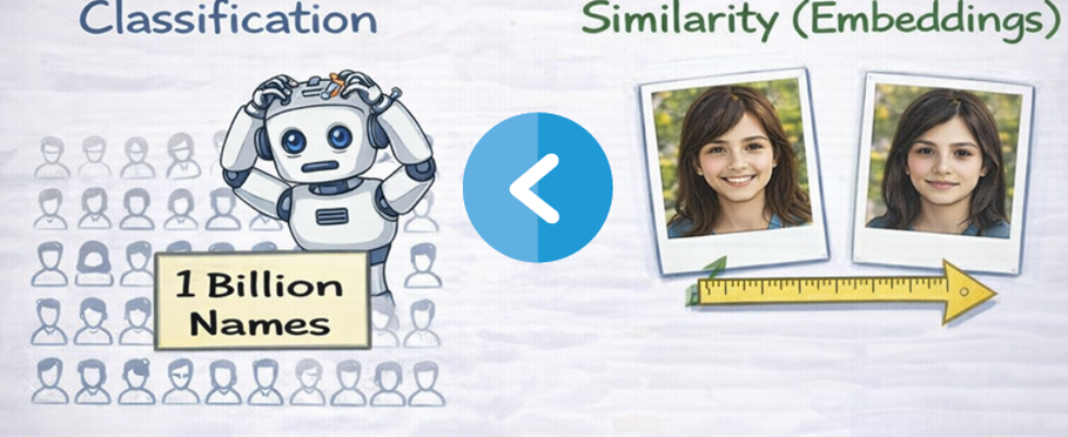
Before we start, you need to know why traditional methods failed. Old-school face recognition treated the problem as classification (assigning a label like ‘Keerthana’ or ‘Mom’ or ‘Dad’).
But that doesn’t scale. Every time you meet a new friend, you’d have to retrain the whole neural network to add a new “class.” For Google, with billions of users, that’s impossible🙅♀️.
So they changed the game by switching to embeddings. Instead of saying ‘This is Keerthana’, the model says, ‘Here is a numerical fingerprint of this face’.

The Working Pipeline

Step 1: Face Detection (Pre-processing)
Before the heavy lifting happens, the system has to actually find the face.
It uses MTCNN (Multi-task Cascaded CNN) or Faster R-CNN to scan the image. The output here isn’t an ID yet; it’s just a bounding box around anything that looks like a human face.
Step 2: Face Alignment
Once we have the box, we need to normalize it. You might be tilting your head or looking sideways, but the model needs consistency.
The system detects facial landmarks (eyes, nose, mouth). It then performs an affine transformation to rotate and scale the face so the eyes are always in a standard position. Finally, it crops the image to a strictly standardized 160×160 pixel size.
Step 3: FaceNet Architecture
Now comes the real deal! The 160×160 input is fed into the deep learning backbone.
The Backbone: Google uses Inception-ResNet-V2. This is one heck of a CNN that combines Inception modules (wide filters) with Residual connections (deep layers).
The Output: This network outputs a 128-dimensional embedding, unlike normal neural networks that output a classification probability.
L2 Normalization: This vector is L2 normalized. Meaning it is projected onto a unit hypersphere.
Why 128 dimensions?
- It is compact enough for fast storage and search.
- It provides enough ‘space’ to distinguish between billions of different faces.
- Because it is on a unit sphere, we can use simple Euclidean distance to compare faces.
Step 4: Triplet Loss Training
How does the network learn which numbers to output? It uses Triplet Loss.
During training, the model looks at three images at once:
1. Anchor (A): A photo of Person X.
2. Positive (P): A different photo of Person X.
3. Negative (N): A photo of Person Y.
The loss function forces the distance between the Anchor and Positive to be smaller than the distance between the Anchor and Negative, plus a margin (α).
The Formula:
Loss = max(0, ||f(A) – f(P)||² – ||f(A) – f(N)||² + margin)
The goal is to push the Positive pair close together and shove the Negative pair away by at least a margin of 0.2.

Step 5: Hard Negative Mining
If you keep picking random strangers as Negatives, the model gets lazy. It’s obv very easy to tell me apart from a 70-year-old man. The loss hits zero too fast, and the model stops learning.
To fix this, Google uses Hard Negative Mining.
They sample ‘Hard Negatives’ i.e. different people who look surprisingly similar to the Anchor. This forces the model to learn fine-grained distinctions (like nose shape or eye spacing) rather than relying on easy features like skin tone.

Step 5: Face Clustering
Once the network is trained, we don’t need to run it again. We just extract the 128D embedding for every face in your library.
The system then runs a clustering algorithm like DBSCAN or agglomerative clustering.
- It groups vectors that are close together in that 128D space.
- Each cluster represents one unique person.
This is why you don’t need to retrain the model for new people. You just add their dot to the graph. If a dot lands in empty space, congratulations! you’ve met a new person.
Edge Cases
It’s not perfect. Things like aging drift (your face changing over 10 years) or extreme alignment failures (weird angles) can still trip it. But with a benchmark accuracy of 99.63% on LFW (Labeled Faces in the Wild), it’s still pretty accurate.

TL;DR: The Tech Stack Summary
For the builders out there, here is the full spec sheet:
- Framework: TensorFlow
- Backbone: Inception-ResNet-V2
- Input: 160×160 RGB images
- Output: 128D L2 normalized embedding
- Loss: Triplet Loss (margin ~0.2) with Hard Negative Mining
- Training Data: 200M+ images (batch size ~1800)
- Clustering: DBSCAN / Agglomerative
- Serving: TensorFlow Lite (on-device)
- Result: 99.63% accuracy on LFW benchmark
It’s not magic. It’s just optimization on a unit hypersphere
ps: I spent way too long reading the original FaceNet paper instead of applying for jobs yesterday, but understanding the shift from Softmax to Triplet Loss was totally worth it.
Thanks a lot for being with me till the end! Means a lot that u’d take your time to read my blogs. See you in the next one! Byeee & sending love 💝
Reverse Engineering Google Photos: FaceNet, Triplet Loss, and Why Softmax is RIP was originally published in Towards AI on Medium, where people are continuing the conversation by highlighting and responding to this story.
