KV Cache in LLM Inference

Why long context eats VRAM, how to estimate it in one line, and what actually fixes it

If you’ve ever tried to run a model with a longer prompt, increased batch size, or enabled beam search and suddenly hit CUDA out-of-memory, there’s a high chance the culprit wasn’t the model weights.

It was the KV cache.

Weights are fixed. KV cache grows with tokens.

So at inference time, memory pressure often comes from the thing you are generating: sequence length.

This article breaks KV cache down into:

• intuition first,
• then exact shapes,
• one formula,
• practical consequences (GQA/MQA, beam search, FP8),
• and a Python tool to estimate it.

1) The intuition: KV cache exists because we refuse to redo work

LLMs generate text one token at a time. At step t, the model generates token t+1 by attending to tokens 1..t.

Self-attention uses three projections of hidden states:

• Q (Query)
• K (Key)
• V (Value)

If you recompute K and V for the entire prefix at every step, you repeat the same matrix multiplications again and again. That’s slow.

So inference engines do the obvious optimization:

Compute Keys and Values once, store them, and reuse them for future tokens.

That stored history is the KV cache.

Student-friendly analogy:

• Writing an essay one sentence at a time.
• -KV cache is your notes staying on the desk.
• Without it, you rewrite your notes before every sentence.

2) What is stored (exactly), and why it grows

For a decoder-only transformer (GPT/LLaMA-style), each layer stores K and V for every past token. Conceptual shapes per layer:

K: [B, Hkv, T, D]
V: [B, Hkv, T, D]

Where:

• B = batch size (often multiplied by beams)
• T = cached tokens so far (prompt + generated)
• Hkv = number of KV heads
• D = head dimension

You store this for every layer.

So the idea is simple:

KV cache is linear in T. Every new token adds more cache.

That’s the “token tax”.

3) Prefill vs Decode

Inference has two phases:

Prefill (processing the prompt)

You feed the entire prompt in one go. The model computes K/V for all prompt tokens and writes them into the cache.

Decode (generating tokens)

You generate one token at a time. Each new token adds one new slice to K/V in every layer.

So memory keeps growing during decode, even when weights stay fixed. That’s why long generation + long context is dangerous.

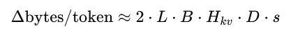
4) The one formula: KV cache memory

Let:

• L = number of layers
• B = batch size
• T = cached tokens (prompt + generated so far)
• Hkv = number of KV heads
• D = head dimension
• s = bytes per element (fp16/bf16=2, fp32=4, fp8=1)

Then approximate KV cache size:

The leading 2 is because you store K and V.

The “token tax” (per generated token)

So memory complexity is O(T) because the cache stores one Key and one Value vector per token (per layer). For a fixed model and dtype, the memory added by each new token is constant.

After T cached tokens, you’ve added that constant T times → memory grows linearly with T. That’s O(T).

5) Why Mistral 7B is the perfect example

Mistral 7B’s public config typically shows:

• 32 layers (num_hidden_layers = 32)
• 32 attention heads (num_attention_heads = 32)
• 8 KV heads (num_key_value_heads = 8) → Grouped-Query Attention (GQA)
• head_dim = 128, hidden_size = 4096
• sliding_window = 4096 (Sliding Window Attention)

And the official Mistral announcement explains the sliding-window mechanism and how stacked layers let information propagate farther than a single layer’s window would suggest.

Transformers’ Mistral docs also describe Mistral as using SWA (trained with an 8K context length) and a fixed cache size, plus GQA for faster inference and lower memory.

That gives you two powerful levers to talk about:

1. GQA reduces KV cache constants (Hkv smaller)
2. SWA can cap cache growth (min(T, W) behavior in implementations that use a rolling cache)

6) KV Cache Memory in Mistral 7B

Let’s plug Mistral 7B’s typical config values into the KV-cache formula:

• Layers: L = 32
• KV heads (GQA): Hkv = 8
• Head dimension: D = 128
• Precision: bf16/fp16 → s = 2 bytes
• Batch: B = 1

Step 1 “Token tax”: how much KV cache one new token adds

Each generated token appends one K and one V vector per layer:

Rule of thumb: for Mistral 7B, batch 1, bf16/fp16, KV cache grows by about 128 KiB per generated token.

Step 2: If attention were “global” (KV grows with all cached tokens T)

If you stored KV for all cached tokens TTT:

So for T = 8192 tokens:

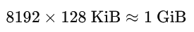
Step 3 : Sliding Window Attention caps effective cache to W

Mistral uses Sliding Window Attention with a window often set to W = 4096. In many implementations, you can keep a rolling cache of size W, so memory scales like:

So once you exceed the window, the cache is effectively capped around:

The multiplier that ruins your day: batch (and beams)

KV cache scales linearly with B:

• B = 8 ⇒ about 8× more KV memory
• With SWA cap: 512 MiB × 8 ≈ 4 GiB

Beam search can multiply effective batch again (implementation-dependent), which is why it can blow up VRAM fast.

7) Why GQA is a “cheat code” for KV cache

In classic multi-head attention (MHA), every attention head has its own K/V, so Hkv = H.

In GQA, you can have many query heads, but fewer KV heads shared across groups, so Hkv < H.

KV cache scales linearly with Hkv, so going from 32 KV heads to 8 KV heads is a clean 4× reduction in KV cache, everything else equal. Mistral’s config makes that explicit via num_key_value_heads.

8) What actually changes KV cache

KV cache scales linearly with each factor:

• Context / cached tokens (T): double T → double KV memory (unless SWA caps it)
• Batch (B): double batch → double KV memory
• Layers (L): deeper model → bigger cache
• KV heads (Hkv): MHA vs GQA/MQA is often the biggest win
• Precision (s): bf16→fp8 can cut cache roughly in half (plus/minus overhead)
• Beam search: often multiplies effective batch → easy OOM

9) Python: KV cache calculator (Mistral-friendly)

If you want a quick estimate for your model/config, this little script is intentionally simple:

It estimates KV cache only, not model weights, activations, allocator overhead, or attention metadata.

In practice, real usage can be a bit higher due to padding/alignment, paged-attention bookkeeping, or quantization scales.

Still, the scaling is the important part:

KV memory grows linearly with T and B, and shrinks linearly with fewer KV heads (GQA) or lower precision.

DTYPE_BYTES = {"fp32": 4, "fp16": 2, "bf16": 2, "fp8": 1}

def pretty_bytes(n: int) -> str:
    units = ["B", "KiB", "MiB", "GiB", "TiB"]
    x = float(n)
    for u in units:
        if x < 1024:
            return f"{x:,.2f} {u}"
        x /= 1024
    return f"{x:,.2f} PiB"

def kv_cache_bytes(L, B, T, Hkv, D, dtype="bf16") -> int:
    # bytes ≈ 2 * L * B * T * Hkv * D * s
    s = DTYPE_BYTES[dtype]
    return 2 * L * B * T * Hkv * D * s

def kv_cache_bytes_swa(L, B, T, W, Hkv, D, dtype="bf16") -> int:
    # Sliding-window implementations can cap the cache to W
    return kv_cache_bytes(L, B, min(T, W), Hkv, D, dtype)

def token_tax_bytes(L, B, Hkv, D, dtype="bf16") -> int:
    s = DTYPE_BYTES[dtype]
    return 2 * L * B * Hkv * D * s

if __name__ == "__main__":
    # Mistral 7B-ish defaults from common configs:
    # L=32, Hkv=8, D=128, W=4096
    L, Hkv, D, W = 32, 8, 128, 4096
    dtype = "bf16"

    for B in [1, 4, 8]:
        print(f"nBatch B={B}")
        print("Per-token KV growth:", pretty_bytes(token_tax_bytes(L, B, Hkv, D, dtype)))

        for T in [1024, 4096, 8192, 16384]:
            full = kv_cache_bytes(L, B, T, Hkv, D, dtype)
            swa  = kv_cache_bytes_swa(L, B, T, W, Hkv, D, dtype)
            print(f"T={T:5d} | global={pretty_bytes(full):>10} | SWA-capped={pretty_bytes(swa):>10}")

10) Fixing OOM in production

If KV cache is your bottleneck, your best levers are:

1. Use a GQA/MQA model (reduce Hkv): Mistral already does this.
2. Use sliding window / capped cache when the architecture supports it: Mistral’s SWA is exactly that idea.
3. Lower KV precision (fp16→fp8/int8 schemes)
4. Reduce batch/beam (often the fastest “stop OOM” switch)
5. Paged/blocked KV storage (doesn’t change scaling, but improves utilization and throughput)

Closing thought

At inference time, weights are fixed but KV cache grows with tokens. The fastest way to reason about VRAM is to remember the token tax:

Each new token adds a constant amount of KV per layer. Mistral 7B makes this especially clear: GQA shrinks the constant, and sliding window attention can cap growth.

If you’re debugging OOMs or trying to scale throughput, start here: reduce T, B/beam, or Hkv, or lower KV precision.

---

KV Cache in LLM Inference was originally published in Towards AI on Medium, where people are continuing the conversation by highlighting and responding to this story.