Hierarchical Clustering: A Tree-Based Approach to Data Grouping

digitado ⋅ 10 de July de 2025

In this blog, you will explore hierarchical clustering in Python, understand its application in machine learning, and review a practical hierarchical clustering example. We will delve into the hierarchical clustering algorithm, compare its implementation in R, and discuss its significance in data mining.

What is Hierarchical Clustering?
Types of Hierarchical Clustering
Agglomerative Clustering Hierarchical
Divisive Hierarchical Clustering
Supervised vs Unsupervised Learning
Why Hierarchical Clustering?
No Need to Pre-specify Number of Clusters
Captures Nested Clusters
Flexibility with Cluster Shapes
Distance Metrics and Linkage Criteria
Handling Outliers
Robustness to Initialization
Visual Interpretation
Practical Example
Steps to Perform Hierarchical Clustering
Setting up the Example
Creating a Proximity Matrix
Steps to Perform Hierarchical Clustering
How to Choose the Number of Clusters in Hierarchical Clustering?
Solving the Wholesale Customer Segmentation Problem
Conclusion

What is Hierarchical Clustering?

Hierarchical clustering is an unsupervised learning technique for grouping similar objects into clusters. It creates a hierarchy of clusters by merging or splitting them based on similarity measures. It uses a bottom-up or top-down approach to construct a hierarchical data clustering schema.

Clustering Hierarchical groups similar objects into a dendrogram. It merges similar clusters iteratively, starting with each data point as a separate cluster. This creates a tree-like structure that shows the relationships between clusters and their hierarchy.

The dendrogram from hierarchical clustering reveals the hierarchy of clusters at different levels, highlighting natural groupings in the data. It provides a visual representation of the relationships between clusters, helping to identify patterns and outliers, making it a valuable tool for exploratory data analysis. For example, let’s say we have the below points, and we want to cluster them into groups:

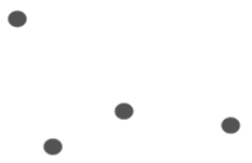
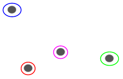
We can assign each of these points to a separate cluster:

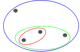
Now, based on the similarity of these clusters, we can combine the most similar clusters and repeat this process until only a single cluster is left:

We are essentially building a hierarchy of clusters. That’s why this algorithm is called hierarchical clustering. I will discuss how to decide the number of clusters later. For now, let’s look at the different types of hierarchical clustering.

Types of Hierarchical Clustering

There are mainly two types of hierarchical clustering:

Agglomerative hierarchical clustering
Divisive Hierarchical clustering

Let’s understand each type in detail.

Agglomerative Clustering Hierarchical

In this technique, we assign each point to an individual cluster. Suppose there are 4 data points. We will assign each of these points to a cluster and hence will have 4 clusters in the beginning:

Then, at each iteration, we merge the closest pair of clusters and repeat this step until only a single cluster is left:

We are merging (or adding) the clusters at each step, right? Hence, this type of clustering is also known as additive hierarchical clustering.

Divisive Hierarchical Clustering

Divisive Clustering Hierarchical works in the opposite way. Instead of starting with n clusters (in case of n observations), we start with a single cluster and assign all the points to that cluster.

So, it doesn’t matter if we have 10 or 1000 data points. All these points will belong to the same cluster at the beginning:

Now, at each iteration, we split the farthest point in the cluster and repeat this process until each cluster only contains a single point:

We are splitting (or dividing) the clusters at each step, hence the name divisive hierarchical clustering.

Agglomerative Clustering is widely used in the industry and will be the article’s focus. Divisive hierarchical clustering will be a piece of cake once we have a handle on the agglomerative type

Applications of Hierarchical Clustering

Here are some common applications of hierarchical clustering:

Biological Taxonomy: Hierarchical clustering is extensively used in biology to classify organisms into hierarchical taxonomies based on similarities in genetic or phenotypic characteristics. It helps understand evolutionary relationships and biodiversity.
Document Clustering: In natural language processing, hierarchical clustering groups similar documents or texts. It aids in topic modelling, document organization, and information retrieval systems.
Image Segmentation: Hierarchical clustering segments images by grouping similar pixels or regions based on colour, texture, or other visual features. It finds applications in medical imaging, remote sensing, and computer vision.
Customer Segmentation: Businesses use hierarchical clustering to group customers into groups based on their purchasing behaviours, demographics, or preferences. This helps with targeted marketing, personalized recommendations, and customer relationship management.
Anomaly Detection: Hierarchical clustering can identify outliers or anomalies in datasets by isolating data points that do not fit well into any cluster. It is useful in fraud detection, network security, and quality control.
Social Network Analysis: Hierarchical clustering helps uncover community structures or hierarchical relationships in social networks by clustering users based on their interactions, interests, or affiliations. It aids in understanding network dynamics and identifying influential users.
Market Basket Analysis: Retailers use hierarchical clustering to analyze transaction data and identify associations between products frequently purchased together. It enables them to optimize product placements, promotions, and cross-selling strategies.

Advantages and Disadvantages of Hierarchical Clustering

Here are some advantages and disadvantages of hierarchical clustering:

Advantages of hierarchical clustering:

Easy to interpret: Hierarchical clustering produces a dendrogram, a tree-like structure that shows the order in which clusters are merged. This dendrogram provides a clear visualization of the relationships between clusters, making the results easy to interpret.
No need to specify the number of clusters: Unlike other clustering algorithms, such as k-means, hierarchical clustering does not require you to specify the number of clusters beforehand. The algorithm determines the number of clusters based on the data and the chosen linkage method.
Captures nested clusters: Hierarchical clustering captures the hierarchical structure in the data, meaning it can identify clusters within clusters (nested clusters). This can be useful when the data naturally forms a hierarchy.
Robust to noise: Hierarchical clustering is robust to noise and outliers because it considers the entire dataset when forming clusters. Outliers may not significantly affect the clustering process, especially if a suitable distance metric and linkage method are chosen.

Disadvantages of hierarchical clustering:

Computational complexity: Hierarchical clustering can be computationally expensive, especially for large datasets. The time complexity of hierarchical clustering algorithms is typically 𝑂(𝑛2log⁡𝑛)O(n2logn) or 𝑂(𝑛3)O(n3), where 𝑛n is the number of data points.
Memory usage: Besides computational complexity, hierarchical clustering algorithms can consume a lot of memory, particularly when dealing with large datasets. Storing the entire distance matrix between data points can require substantial memory.
Difficulty with large datasets: Due to its computational complexity and memory requirements, hierarchical clustering may not be suitable for large datasets. In such cases, alternative clustering methods, such as k-means or DBSCAN, may be more appropriate.
Sensitive to noise and outliers: While hierarchical clustering is generally robust to noise and outliers, extreme outliers or noise points can still affect the clustering results, especially if they are not handled properly beforehand.
Difficulty in merging clusters: Once clusters are formed in hierarchical clustering, merging or splitting them can be difficult, especially if the clustering uses a divisive method. This lack of flexibility can be a limitation in certain scenarios where cluster adjustments are needed.

Application of Hierarchical Clustering with Python

In Python, the scipy and scikit-learn libraries are often used to perform hierarchical clustering. Here’s how you can apply hierarchical clustering using Python:

Import Necessary Libraries: First, you’ll need to import the necessary libraries: numpy for numerical operations, matplotlib for plotting, and scipy.cluster.hierarchy for hierarchical clustering.
Generate or Load Data: You can generate a synthetic dataset or load your dataset.
Compute the Distance Matrix: Compute the distance matrix, which will be used to form clusters.
Perform Hierarchical Clustering: Use the linkage method to perform hierarchical clustering.
Plot the Dendrogram: Visualize the clusters using a dendrogram.

Here’s an example of hierarchical clustering using Python:

import numpy as np

import matplotlib.pyplot as plt
from scipy.cluster.hierarchy import dendrogram, linkage

from scipy.cluster.hierarchy import fcluster

from sklearn.datasets import make_blobs

# Generate sample data

X, y = make_blobs(n_samples=100, centers=3, cluster_std=0.60, random_state=0)

# Compute the linkage matrix

Z = linkage(X, 'ward')

# Plot the dendrogram

plt.figure(figsize=(10, 7))

plt.title("Dendrogram")

plt.xlabel("Sample index")

plt.ylabel("Distance")

dendrogram(Z)

plt.show()

# Determine the clusters

max_d = 7.0 # this can be adjusted based on the dendrogram

clusters = fcluster(Z, max_d, criterion='distance')

# Plot the clusters

plt.figure(figsize=(10, 7))

plt.scatter(X[:, 0], X[:, 1], c=clusters, cmap='prism')

plt.title("Hierarchical Clustering")

plt.xlabel("Feature 1")

plt.ylabel("Feature 2")

plt.show()Copy Code

Supervised vs Unsupervised Learning

Understanding the difference between supervised and unsupervised learning is important before we dive into the Clustering hierarchy. Let me explain this difference using a simple example.

Suppose we want to estimate the count of bikes that will be rented in a city every day:

Or, let’s say we want to predict whether a person on board the Titanic survived or not:

Examples

In the first example, we have to predict the number of bikes based on features like the season, holiday, working day, weather, and temperature.
In the second example, we are predicting whether a passenger survived. In the ‘Survived’ variable, 0 represents that the person did not survive, and one means the person did make it out alive. The independent variables here include Pclass, Sex, Age, Fare, etc.

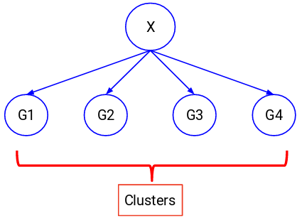
Let’s look at the figure below to understand this visually:

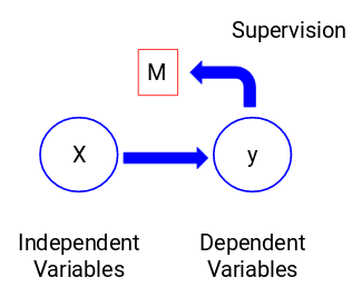
Here, y is our dependent or target variable, and X represents the independent variables. The target variable is dependent on X, also called a dependent variable. We train our model using the independent variables to supervise the target variable. Hence, the name supervised learning.

When training the model, we aim to generate a function that maps the independent variables to the desired target. Once the model is trained, we can pass new sets of observations, and the model will predict their target. This, in a nutshell, is supervised learning.

In these cases, we try to divide the entire data into a set of groups. These groups are known as clusters, and the process of making them is known as clustering.

This technique is generally used to cluster a population into different groups. Some common examples include segmenting customers, clustering similar documents, and recommending similar songs or movies.

There are many more applications of unsupervised learning. If you come across any interesting ones, feel free to share them in the comments section below!

Various algorithms help us make these clusters. The most commonly used clustering algorithms are K-means and Hierarchical clustering.

Why Hierarchical Clustering?

We should first understand how K-means works before we explore hierarchical clustering. Trust me, it will make the concept much easier.

Here’s a brief overview of how K-means works:

Decide the number of clusters (k)
Select k random points from the data as centroids
Assign all the points to the nearest cluster centroid
Calculate the centroid of newly formed clusters
Repeat steps 3 and 4

It is an iterative process. It will continue until the centroids of newly formed clusters do not change or the maximum number of iterations is reached.

However, there are certain challenges with K-means. It always tries to make clusters of the same size. Also, we have to decide the number of clusters at the beginning of the algorithm. Ideally, we would not know how many clusters we should have at the beginning of the algorithm, and hence, it is a challenge with K-means.

This is a gap hierarchical clustering bridge with aplomb. It takes away the problem of having to pre-define the number of clusters. Sounds like a dream! So, let’s see what hierarchical clustering is and how it improves on K-means.

How Does Hierarchical Clustering Improve on K-means?

Hierarchical clustering and K-means are popular clustering algorithms with different strengths and weaknesses. Here are some ways in which hierarchical clustering can improve on K-means:

No Need to Pre-specify Number of Clusters

Hierarchical Clustering:

Does not require the number of clusters (k) to be specified in advance.
The dendrogram provides a visual representation of the hierarchy of clusters, and the number of clusters can be determined by cutting the dendrogram at a desired level.

K-means:

It requires specifying the number of clusters (k) beforehand, which can be difficult if the optimal number of clusters is unknown.

Captures Nested Clusters

Hierarchical Clustering:

It can identify nested clusters, meaning it can find clusters within them.
This is useful for datasets with a natural hierarchical structure (e.g., taxonomy of biological species).

K-means:

Assumes clusters are flat and do not capture hierarchical relationships.

Flexibility with Cluster Shapes

Hierarchical Clustering:

Can find clusters of arbitrary shapes.
The algorithm is not restricted to spherical clusters and can capture more complex cluster structures.

K-means:

Assumes clusters are spherical and of similar size, which may not be suitable for datasets with irregularly shaped clusters.

Distance Metrics and Linkage Criteria

Hierarchical Clustering:

Offers flexibility in distance metrics (e.g., Euclidean, Manhattan) and linkage criteria (e.g., single, complete, average).
This flexibility can improve clustering performance on different types of data.

K-means:

Typically, it uses the Euclidean distance, which may not be suitable for all data types.

Handling Outliers

Hierarchical Clustering:

Outliers can be identified as singleton clusters at the bottom of the dendrogram.
This makes it easier to detect and potentially remove outliers.

K-means:

Sensitive to outliers, as they can significantly affect the position of cluster centroids.

Robustness to Initialization

Hierarchical Clustering:

Does not require random initialization of cluster centroids.
The clustering result is deterministic and does not depend on initial conditions.

K-means:

Requires random initialization of centroids, leading to different clustering results in different runs.
The algorithm may converge to local minima, depending on the initial placement of centroids.

Visual Interpretation

Hierarchical Clustering:

The dendrogram provides a visual and interpretable representation of the clustering process.
It helps in understanding the relationships between clusters and the data structure.

K-means:

Provides cluster labels and centroids but does not visually represent the clustering process.

Practical Example

Let’s consider a practical example using hierarchical clustering and K-means on a simple dataset:

import numpy as np

import matplotlib.pyplot as plt

from scipy.cluster.hierarchy import dendrogram, linkage

from sklearn.datasets import make_blobs

from sklearn.cluster import KMeans

# Generate sample data

X, y = make_blobs(n_samples=100, centers=3, cluster_std=0.60, random_state=0)

# Hierarchical Clustering

Z = linkage(X, 'ward')

plt.figure(figsize=(10, 7))

plt.title("Hierarchical Clustering Dendrogram")

dendrogram(Z)

plt.show()

# K-means Clustering

kmeans = KMeans(n_clusters=3, random_state=0).fit(X)

labels = kmeans.labels_

plt.figure(figsize=(10, 7))

plt.scatter(X[:, 0], X[:, 1], c=labels, cmap='prism')

plt.title("K-means Clustering")

plt.show()Copy Code

Steps to Perform Hierarchical Clustering

We know that in hierarchical clustering, we merge the most similar points or clusters. Now the question is: How do we decide which points are similar and which are not? It’s one of the most important questions in clustering!

Here’s one way to calculate similarity — Take the distance between the centroids of these clusters. The points with the least distance are referred to as similar points, and we can merge them. We can also refer to this as a distance-based algorithm (since we are calculating the distances between the clusters).

In hierarchical clustering, we have a concept called a proximity matrix. This stores the distances between each point. Let’s take an example to understand this matrix and the steps to perform hierarchical clustering.

Setting up the Example

Suppose a teacher wants to divide her students into different groups. She has the marks scored by each student in an assignment, and based on these marks, she wants to segment them into groups. There’s no fixed target here as to how many groups to have. Since the teacher does not know what type of students should be assigned to which group, it cannot be solved as a supervised learning problem. So, we will try to apply hierarchical clustering here and segment the students into different groups.

Let’s take a sample of 5 students:

Creating a Proximity Matrix

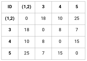
First, we will create a proximity matrix that tells us the distance between each of these points. Since we are calculating the distance of each point from each of the other points, we will get a square matrix of shape n X n (where n is the number of observations).

Let’s make the 5 x 5 proximity matrix for our example:

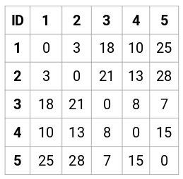
The diagonal elements of this matrix will always be 0 as the distance of a point with itself is always 0. We will use the Euclidean distance formula to calculate the rest of the distances. So, let’s say we want to calculate the distance between points 1 and 2:

√(10–7)² = √9 = 3

Similarly, we can calculate all the distances and fill the proximity matrix.

Steps to Perform Hierarchical Clustering

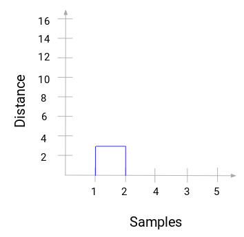
Step 1: First, we assign all the points to an individual cluster:

Different colours here represent different clusters. You can see that we have 5 different clusters for the 5 points in our data.

Step 2: Next, we will look at the smallest distance in the proximity matrix and merge the points with the smallest distance. We then update the proximity matrix:

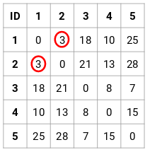
Here, the smallest distance is 3 and hence we will merge point 1 and 2:

Let’s look at the updated clusters and accordingly update the proximity matrix:

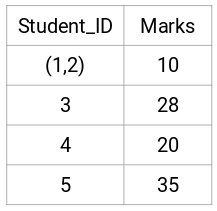
Here, we have taken the maximum of the two marks (7, 10) to replace the marks for this cluster. Instead of the maximum, we can also take the minimum value or the average values as well. Now, we will again calculate the proximity matrix for these clusters:

Step 3: We will repeat step 2 until only a single cluster is left.

So, we will first look at the minimum distance in the proximity matrix and then merge the closest pair of clusters. We will get the merged clusters as shown below after repeating these steps:

We started with 5 clusters and finally had a single cluster. This is how agglomerative hierarchical clustering works. But the burning question remains — how do we decide the number of clusters? Let’s understand that in the next section.

How to Choose the Number of Clusters in Hierarchical Clustering?

Are you ready to finally answer this question that has been hanging around since we started learning? To get the number of clusters for hierarchical clustering, we use an awesome concept called a Dendrogram.

A dendrogram is a tree-like diagram that records the sequences of merges or splits.

Example

Let’s get back to the teacher-student example. Whenever we merge two clusters, a dendrogram will record the distance between them and represent it in graph form. Let’s see how a dendrogram looks:

We have the samples of the dataset on the x-axis and the distance on the y-axis. Whenever two clusters are merged, we will join them in this dendrogram, and the height of the join will be the distance between these points. Let’s build the dendrogram for our example:

Take a moment to process the above image. We started by merging samples 1 and 2, and the distance between these two samples was 3 (refer to the first proximity matrix in the previous section). Let’s plot this in the dendrogram:

Here, we can see that we have merged samples 1 and 2. The vertical line represents the distance between these samples. Similarly, we plot all the steps where we merged the clusters, and finally, we get a dendrogram like this:

We can visualize the steps of hierarchical clustering. The more the distance of the vertical lines in the dendrogram, the more the distance between those clusters.

Now, we can set a threshold distance and draw a horizontal line (Generally, we try to set the threshold so that it cuts the tallest vertical line). Let’s set this threshold as 12 and draw a horizontal line:

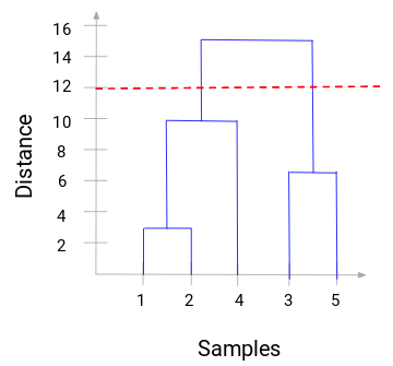
The number of clusters will be the number of vertical lines intersected by the line drawn using the threshold. In the above example, since the red line intersects two vertical lines, we will have 2 clusters. One cluster will have a sample (1,2,4), and the other will have a sample (3,5).

Solving the Wholesale Customer Segmentation Problem

We will be working on a wholesale customer segmentation problem. You can download the dataset using this link. The data is hosted on the UCI Machine Learning repository. This problem aims to segment a wholesale distributor’s clients based on their annual spending on diverse product categories, like milk, grocery, region, etc.

Let’s explore the data first and then apply Hierarchical Clustering to segment the clients.

Python Code

import pandas as pd
import numpy as np
import matplotlib.pyplot as plt
#%matplotlib inline
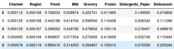
data = pd.read_csv('Wholesale customers data.csv')
print(data.head())Copy Code

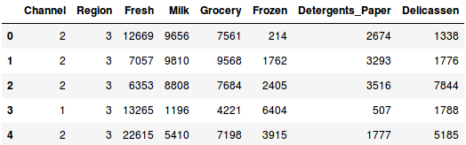
There are multiple product categories — fresh, Milk, Grocery, etc. The values represent the number of units each client purchases for each product. We aim to make clusters from this data to segment similar clients. Of course, we will use Hierarchical Clustering for this problem.

But before applying, we have to normalize the data so that the scale of each variable is the same. Why is this important? If the scale of the variables is not the same, the model might become biased towards the variables with a higher magnitude, such as fresh or milk (refer to the above table).

So, let’s first normalize the data and bring all the variables to the same scale:

from sklearn.preprocessing import normalize
data_scaled = normalize(data)
data_scaled = pd.DataFrame(data_scaled, columns=data.columns)
data_scaled.head()

Here, we can see that the scale of all the variables is almost similar. Now, we are good to go. Let’s first draw the dendrogram to help us decide the number of clusters for this particular problem:

import scipy.cluster.hierarchy as shc
plt.figure(figsize=(10, 7))  
plt.title("Dendrograms")  
dend = shc.dendrogram(shc.linkage(data_scaled, method='ward'))

The x-axis contains the samples and y-axis represents the distance between these samples. The vertical line with maximum distance is the blue line and hence we can decide a threshold of 6 and cut the dendrogram:

plt.figure(figsize=(10, 7))  
plt.title("Dendrograms")  
dend = shc.dendrogram(shc.linkage(data_scaled, method='ward'))
plt.axhline(y=6, color='r', linestyle='--')

We have two clusters as this line cuts the dendrogram at two points. Let’s now apply hierarchical clustering for 2 clusters:

from sklearn.cluster import AgglomerativeClustering
cluster = AgglomerativeClustering(n_clusters=2, affinity='euclidean', linkage='ward')  
cluster.fit_predict(data_scaled)

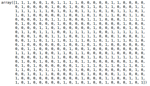
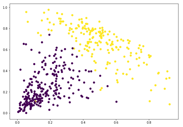
We can see the values of 0s and 1s in the output since we defined 2 clusters. 0 represents the points that belong to the first cluster and 1 represents points in the second cluster. Let’s now visualize the two clusters:

plt.figure(figsize=(10, 7))  
plt.scatter(data_scaled['Milk'], data_scaled['Grocery'], c=cluster.labels_)

Conclusion

In our journey, we’ve uncovered a powerful tool for unraveling the complexities of data relationships. From the conceptual elegance of dendrograms to their practical applications in diverse fields like biology, document analysis, cluster analysis, and customer segmentation, hierarchical cluster analysis emerges as a guiding light in the labyrinth of data exploration.

As we conclude this expedition, we stand at the threshold of possibility, where every cluster tells a story, and every dendrogram holds the key to unlocking the secrets of data science. In the ever-expanding landscape of Python and machine learning, hierarchical clustering stands as a stalwart companion, guiding us toward new horizons of discovery and understanding.

Hierarchical clustering is a powerful algorithm in machine learning used for grouping data into a tree-like structure. For example, implementing hierarchical clustering in Python allows users to visualize relationships among data points effectively. This technique is also applicable in R and is widely used in data mining to analyze complex datasets.

Like 0

Liked Liked