
From Embeddings to Intelligence: Vector Aggregate Functions in Snowflake
Embeddings are frequently described as the foundation of modern AI systems, yet they are often treated as a black box. They capture meaning, enable semantic search, and power intelligent applications, but we rarely see how they behave as data or how they can be used analytically in a governed, scalable way.
With the recent introduction of vector aggregate functions in Snowflake, embeddings are no longer just intermediate artifacts but become truly composable building blocks for analytics and AI. By making embeddings and vectors first-class citizens of the data platform, through native VECTOR support, Snowflake Cortex embedding functions, and vector aggregate functions (VECTOR_SUM, VECTOR_AVG, VECTOR_MIN, and VECTOR_MAX), semantic intelligence can now be built directly in SQL, without external pipelines, vector databases, or custom ML infrastructure.
In this blog, I will walk through a semantic support ticket classification workflow, beginning with loading ticket data and generating embeddings in SQL, aggregating them using vector functions (VECTOR_SUM), and finally exposing the results through a Streamlit app, with a clear explanation of what is happening at every step and why the outcomes behave as they do.
The Problem: Text Is Messy, Intent Is Not
Customer support tickets arrive as free-form text written in many different styles. One customer may say “Payment failed but money was deducted,” another may say “Charged twice for the same invoice,” and a third may complain that a refund has not yet arrived. The wording varies, but the underlying intent is clearly related to billing.
Traditional approaches rely on keyword rules or manually trained classifiers. These approaches struggle as language evolves, overlap between categories increases, and maintenance costs grow. What remains consistent, however, is intent. If we can model intent directly, classification becomes far more robust.
The Use Case: Semantic Support Ticket Classification
Imagine a customer support system receiving hundreds or thousands of tickets every day. Each ticket contains free-form text describing an issue.
Traditional approaches rely on keyword rules, regex patterns, and manually trained classifiers. These approaches struggle with variations in wording, ambiguous language, and the ongoing effort required to maintain them over time. Instead, we will build a semantic classification system that understands intent, not just words.

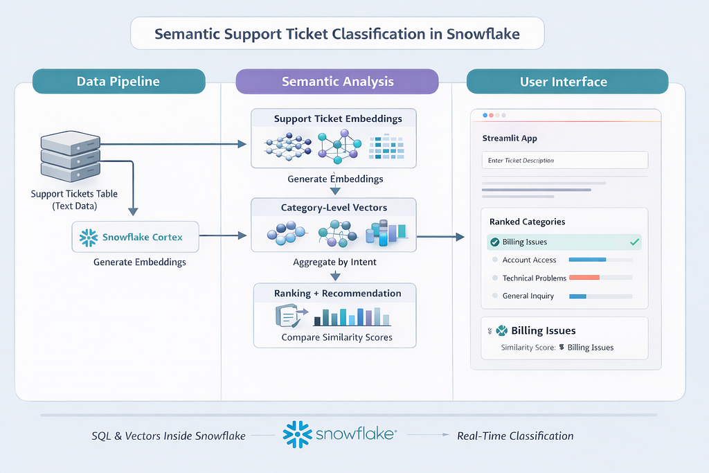
This above illustration shows how raw support ticket text flows through the Snowflake AI Data Cloud, where Snowflake Cortex converts each ticket into an embedding and vector aggregate functions combine individual embeddings into category-level semantic vectors. New tickets are then embedded and compared against these category vectors using cosine similarity, allowing intent-based classification to happen entirely within Snowflake and be surfaced through a Streamlit app. This flow will become clearer as we walk through each step of the implementation in the sections that follow.
Before we Begin: Understanding Embeddings
Before we write any SQL, it is important to understand what embeddings really are. Not conceptually, but practically.
When we say “we generate embeddings”, what are we actually storing?
From Text to Numbers:
An embedding is a numerical representation of text. Instead of treating text as characters or keywords, embeddings represent meaning using numbers.
For example, consider these two support tickets:
“Payment failed but the amount was deducted”
“Money was charged even though the transaction did not complete”
They use different words, but describe the same intent.
An embedding model converts each sentence into a fixed-length vector of numbers that captures this semantic meaning. Think of embeddings like coordinates in a high-dimensional space:
- Each sentence becomes a point
- Semantically similar sentences land close together
- Unrelated sentences are far apart
You never interpret individual numbers. You interpret distance and similarity between vectors.
What an Embedding Vector Looks Like
For example, when Snowflake Cortex generates an embedding using EMBED_TEXT_768 function, it produces something like this:
[ 0.0123, -0.8471, 0.3329, 0.1044, …, -0.2291 ]
In reality:
- This vector has 768 floating-point values
- Each value represents one learned semantic dimension
- Stored natively as VECTOR(FLOAT, 768) in Snowflake
You don’t query these numbers directly. You use vector functions to compare them.
Same Meaning, Similar Vectors
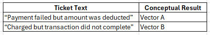
Vector A and Vector B will have:
- High cosine similarity
- Low distance
- Strong semantic alignment
Even though the wording is different.
Different Meaning, Distant Vectors

Vector A and Vector C will be:
- Far apart in vector space
- Lower similarity score than between Vectors A and B
- Clearly separable by intent
A Simple Example
Let us try to understand this using a simple toy example.
Imagine embeddings had only 3 numbers instead of 768, just for illustration.
A billing ticket like: “My credit card was charged twice for the same invoice”
might be represented as: [0.8, 0.6, 0.1]
Now, consider another billing ticket with different wording,
“I was billed twice and the duplicate charge was not refunded”,
could look like: [0.7, 0.5, 0.2]
The numbers are different, but the pattern is similar, so the vectors point in a similar direction and produce a high cosine similarity.
A login-related ticket such as:
“I cannot log into my account after resetting my password”
might look like: [0.1, 0.2, 0.9]
Here the pattern is very different, so the similarity drops.
This is how embeddings compare meaning using patterns of numbers rather than exact matches.
Below is a representative simplified projection of embedding space where descriptions with similar intent appear closer together, while unrelated issues are farther apart.

A useful mental model is to imagine clusters forming naturally. Billing-related tickets cluster in one region, login-related tickets in another, and product issues elsewhere. These clusters emerge automatically from the embedding model, without any rules or labels. This idea, that meaning becomes measurable once text is embedded, is the foundation for everything that follows.
How Snowflake Cortex Fits In
Snowflake Cortex lets us generate these embeddings directly inside SQL:
- No external ML services
- No Python pipelines
- No vector databases
The output embeddings are stored as a first-class Snowflake data type, which means they can be queried, aggregated, and compared using standard SQL. This tight integration allows semantic intelligence to be built as part of normal analytical workflows, with full governance, scalability, and operational simplicity.
The Process Flow and Step-by-Step Implementation
The architecture follows a clean, Snowflake-native flow that keeps all semantic intelligence inside the data platform.
Step 1: Support ticket text is first stored in a structured table in Snowflake.
Step 2: The ticket text is passed to Snowflake Cortex, where embeddings are generated directly using a built-in embedding model.
Step 3: These ticket-level embeddings are then aggregated by issue category using vector aggregate functions to produce category-level semantic vectors that represent collective intent.
Step 4: When a new ticket arrives, it is embedded using the same model and compared against the category vectors using cosine similarity, enabling intent-based classification entirely in SQL.
Step 5: A Snowflake-native Streamlit app sits on top of this workflow as a thin user interface, allowing users to submit ticket text and view ranked category recommendations in real time, while all computation, governance, and scaling remain handled within Snowflake.
With this end-to-end flow in mind, we will get into the details for each step. We begin by loading the support ticket data into Snowflake in Step 1.
Step 1: Load the Support Tickets Dataset
We start by creating structured table containing raw ticket text and known categories. The dataset provided (support_tickets.csv) consists of multiple categories, with varied phrasing within categories.
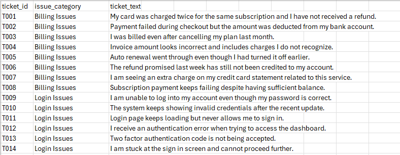
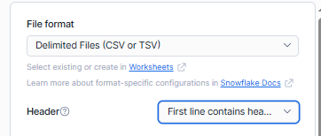
Load the above file using Snowsight and create the SUPPORT_TICKETS table.

Before loading ensure that you are selecting the “First line contains headers” option for the Header.
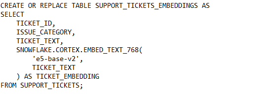
Step 2: Generating Embeddings with Snowflake Cortex
Now we will transform raw text into embeddings using Snowflake Cortex. Each ticket description is passed through an embedding model and stored as a vector inside Snowflake.
After this step, every ticket has both human-readable text and a machine-readable semantic representation. Tickets describing similar problems already sit closer together in vector space, even though we have not yet performed any aggregation or classification.
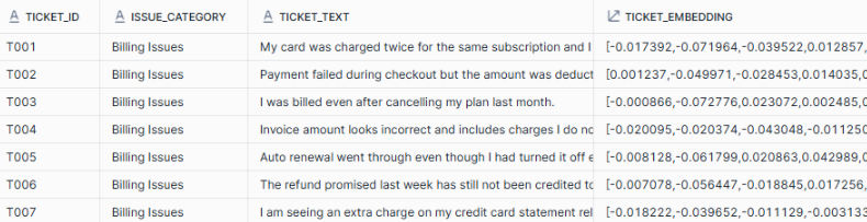
If you inspect this table, you will see that each row now contains a VECTOR(768) column. While the vector values themselves are opaque, their relative similarity is what matters.
Now that embeddings exist at the ticket level, a natural question arises: should we classify new tickets by comparing them against every historical ticket? In practice, though this might work for smaller datasets, it quickly becomes inefficient and difficult to interpret. Instead, we shift from document-level reasoning to category-level reasoning by aggregating embeddings into a single semantic representation per issue category.
Step 3: Aggregating Embeddings into Category-Level Vectors
Snowflake’s vector aggregate function allows us to combine multiple embeddings into a single semantic representation per category. By summing vectors dimension by dimension, we create a category-level vector that captures collective intent.


In this step, VECTOR_SUM combines the embeddings of all tickets within the same issue category. You can think of each embedding as a numerical representation of a ticket’s meaning, and VECTOR_SUM adds these representations together across all tickets in the category. The resulting vector captures the shared intent of the group rather than the details of any single ticket. This aggregated vector acts as a semantic reference for the category and allows new tickets to be compared against categories instead of individual examples, making classification both faster and more stable.
As evident, the result of this query is one row per issue category. Each row contains a vector that represents the semantic center of that category. Instead of dozens of ticket-level embeddings, we now have a compact, interpretable set of semantic anchors.
Step 4: Classifying a New Ticket Using Cosine Similarity
Once we have a semantic vector representing each issue category, the remaining question is how to measure how well a new ticket aligns with those categories. This is where cosine similarity comes in. Rather than comparing exact values, cosine similarity measures how closely two vectors point in the same direction in semantic space. In practical terms, it tells us how similar the meaning of two pieces of text is, independent of how long or detailed they are.
This makes cosine similarity especially well suited for embeddings. Two texts that express the same intent using different words will produce vectors that are oriented similarly, resulting in a high similarity score. Texts that describe different kinds of problems will point in different directions and yield much lower scores. Snowflake’s cosine similarity function handles this comparison directly on VECTOR columns and internally accounts for vector magnitude, so no manual normalization is required.
With this intuition in mind, we can now embed a new incoming support ticket and compare it against each category-level vector to determine the closest semantic match.


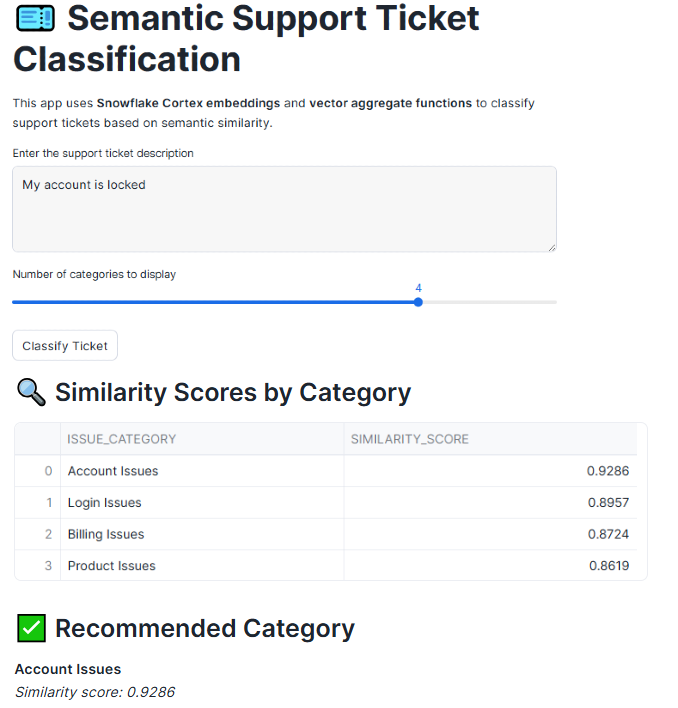
As expected, Billing Issues emerges as the top match with a similarity score of approximately 0.91, clearly ranking above all other categories. This confirms that the aggregated billing vector is capturing the dominant financial intent correctly.
What is interesting and important to understand is that the remaining categories still show relatively high similarity scores rather than collapsing toward zero. Account Issues, Login Issues, and Product Issues all fall in the 0.82–0.84 range. This behavior is not a flaw. It reflects how embeddings model language in the real world. Financial issues often co-occur conceptually with account status, access, and product behavior, and the embedding space captures this shared semantic context.
Cosine similarity measures directional alignment in semantic space, not exclusivity. Even a tightly scoped billing complaint still contains broader notions of user interaction, service behavior, and system outcomes. Because the category vectors are aggregates of many tickets, they represent generalized intent rather than narrow keywords. As a result, related categories retain moderate similarity while the most relevant category still ranks highest.
The key takeaway is that classification is driven by relative ranking, not absolute thresholds. The system correctly identifies Billing Issues as the strongest semantic match, while preserving a realistic gradient of similarity across other categories. In production scenarios, this ranked output can be used both for automatic routing and as a confidence signal. A clear top result indicates high confidence, while closely spaced scores may justify manual review or multi-category routing.
This result demonstrates that vector aggregation produces stable, interpretable behavior that aligns well with how users actually describe problems, rather than forcing artificially sharp boundaries between issue types.
With the semantic classification logic in place, the next step is to make this intelligence accessible to end users through an interactive application.
Step 5: Adding a Streamlit Application Layer
Streamlit provides the interaction layer that makes semantic intelligence accessible to users. By adding a Snowflake-native Streamlit app, we turn a purely analytical workflow into a real-time experience where support agents or analysts can paste in a ticket description and immediately see how it aligns with each issue category.
Let us create the “Semantic Ticket Intelligence” streamlit application.

The application acts as a lightweight interface that orchestrates embedding generation and vector similarity queries directly inside Snowflake. When a user enters ticket text and submits it, the Streamlit app generates an embedding using the same Cortex model used for historical tickets. This ensures the new ticket exists in the same semantic space as the category vectors. The app then executes a cosine similarity query against the aggregated category vectors, retrieves the ranked results, and displays both the similarity scores and the recommended category. Streamlit serves as a thin native presentation layer, while all intelligence lives inside Snowflake.
Together, SQL, vectors, and Streamlit form a cohesive pattern for building semantic applications directly inside the platform. SQL provides the governance, scalability, and familiarity that data teams rely on, vectors introduce a way to reason about meaning rather than keywords, and Streamlit turns this intelligence into an experience that users can interact with in real time.
Beyond VECTOR_SUM: Other Vector Aggregate Functions
In addition to VECTOR_SUM, Snowflake provides other vector aggregate functions: VECTOR_AVG, VECTOR_MIN, and VECTOR_MAX , that allow embeddings to be summarized in different ways. While all of these functions operate on vectors dimension by dimension, each one highlights a different aspect of the underlying semantic data, depending on whether you want to emphasize dominant patterns, typical meaning, or semantic boundaries.
In the support ticket dataset used throughout this blog, each issue category contains multiple tickets describing similar problems using different language. Vector aggregate functions allow us to summarize these ticket-level embeddings into category-level representations, but the choice of function determines how that collective meaning is captured.
As we saw in the illustrated example, VECTOR_SUM combines the embeddings of all tickets in a category by adding them together dimension by dimension. In the context of support tickets, this reinforces semantic signals that appear repeatedly, such as financial terms in billing issues or authentication language in login issues. As a result, the aggregated vector strongly reflects the dominant intent of the category, making VECTOR_SUM particularly well suited for operational tasks like ticket classification and auto-routing.
VECTOR_AVG takes a different approach by averaging embeddings rather than accumulating them. Applied to support tickets, this produces a more neutral representation of what a typical ticket in a category looks like. This can be useful when categories vary significantly in volume or when you want to compare categories without allowing more frequent issues to dominate the representation.
VECTOR_MIN and VECTOR_MAX capture the lower and upper bounds of semantic variation within each category. In a support context, these functions help surface edge cases and outliers, such as tickets that stretch the usual meaning of a category or introduce new issue patterns. While they are less commonly used for direct classification, they provide valuable insight into how broadly or narrowly customers are describing problems within each category.
Together, these vector aggregate functions allow teams to move beyond simple classification and gain a deeper understanding of customer issues. Whether the goal is robust routing, balanced analysis, or exploratory insight, they provide flexible ways to reason about meaning at scale, using the same support ticket data and entirely within Snowflake.
In conclusion, without vector aggregation, embeddings remain as artifacts used primarily for search. With vector aggregation, embeddings become analytical building blocks. We move from document-level reasoning to intent-level reasoning, enabling faster queries, lower cost, better explainability, and cleaner analytics workflows. By keeping embeddings, aggregation, and similarity logic native to Snowflake, this approach avoids fragmented pipelines and external dependencies, allowing semantic intelligence to live where the data already exists. The result is not just a working demo, but a repeatable pattern for building explainable, production-ready AI applications in the AI data cloud.
The end-to-end code associated with this blog can be accessed here.
I share hands-on, implementation-focused perspectives on Snowflake, Cortex AI, LLMs, generative and agentic AI, translating advanced capabilities into practical, real-world analytics use cases. Do follow me on LinkedIn and Medium for more such insights.
From Embeddings to Intelligence: Vector Aggregate Functions in Snowflake was originally published in Towards AI on Medium, where people are continuing the conversation by highlighting and responding to this story.