Fine-Tuning LLMs: A Comprehensive Tutorial
It costs millions of dollars and months of computing time to train a large language model from the ground up. You most likely never need to do it. Fine-tuning lets you adapt pre-trained language models to your needs in hours or days, not months, with a fraction of the resources.
This tutorial takes you from theory to practice: you’ll learn the four core fine-tuning techniques, code a complete training pipeline in Python, and learn the techniques that separate production-ready models from expensive experiments.
What Is LLM Fine-Tuning?
Fine-tuning trains an existing language model on your data to enhance its performance on specific tasks. Pre-trained models are powerful generalists, but exposing them to focused examples can transform them into specialists for your use case.
Instead of building a model from scratch (which requires massive compute and data), you’re giving an already-capable model a crash course in what matters to you, whether that’s medical diagnosis, customer support automation, sentiment analysis, or any other particular task.
How Does LLM Fine-Tuning Work?
Fine-tuning continues the training process on pre-trained language models using your specific dataset. The model processes your provided examples, compares its own outputs to the expected results, and updates internal weights to adapt and minimize loss.
This approach can vary based on your goals, available data, and computational resources. Some projects require full fine-tuning, where you update all model parameters, while others work better with parameter-efficient methods like LoRA that modify only a small subset.
LLM Fine-Tuning Methods
Supervised Fine-Tuning
SFT teaches the model to learn the patterns of the correct question-answer pairs and adjusts model weights to match those answers exactly. You need a dataset of (Prompt, Ideal Response) pairs. Use this when you want consistent outputs, like making the model always respond in JSON format, following your customer service script, or writing emails in your company’s tone.
Unsupervised Fine-Tuning
Feeds the model tons of raw text (no questions or labeled data needed) so it learns the vocabulary and patterns of a particular domain. While this is technically a pre-training process known as Continued Pre-Training (CPT), this is usually done after the initial pre-training phase. Use this first when your model needs to understand specialized content it wasn’t originally trained on, like medical terminology, legal contracts, or a new language.
Direct Preference Optimization
DPO teaches the model to prefer better responses by showing examples of good vs. bad answers to the same question and adjusting it to favor the good ones. Needs (Prompt, Good Response, Bad Response) triplets. Use DPO after basic training to fix annoying behaviors like stopping the model from making things up, being too wordy, or giving unsafe answers.
Reinforcement Fine-Tuning
In RLHF, you first train a reward model on prompts with multiple responses ranked by humans, teaching it to predict which responses people prefer. Then, you use reinforcement learning to optimize and fine-tune a model that generates responses, which the reward model judges. This helps the model learn over time to produce higher-scoring outputs. This process requires datasets in this format: (Prompt, [Response A, Response B, ...], [Rankings]). It’s best for tasks where judging quality is easier than creating perfect examples, like medical diagnoses, legal research, and other complex domain-specific reasoning.
Step-by-Step Fine-Tuning LLMs Tutorial
We’ll walk you through every step of fine-tuning a small pre-trained model to solve word-based math problems, something it struggles with out of the box. We’ll use the Qwen 2.5 base model with 0.5B parameters that already has natural language processing capabilities.
The approach works for virtually any use case of fine-tuning LLMs: teaching a model specialized terminology, improving the model’s performance on specific tasks, or adapting it to your domain.
Prerequisites
Install a few Python packages that we’ll use throughout this tutorial. In a new project folder, create and activate a Python virtual environment, and then install these libraries using pip or your preferred package manager:
pip install requests datasets transformers 'transformers[torch]'
1. Get & Load the Dataset
The fine-tuning process starts with choosing the dataset, which is arguably the most important decision. The dataset should directly reflect the task you want your model to perform.
Simple tasks like sentiment analysis need basic input-output pairs. Complex tasks like instruction following or question-answering require richer datasets with context, examples, and varied formats. Fine-tuning data quality and size directly impact training time and your model’s performance.
The easiest starting point is the Hugging Face dataset library, which hosts thousands of open-source datasets for different domains and tasks. Need something specific and high-quality? Purchase specialized datasets or build your own by scraping publicly available data.
For example, if you want to build a sentiment analysis model for Amazon product reviews, you may want to collect data from real reviews using a web scraping tool. Here’s a simple example that uses Oxylabs Web Scraper API:
import json
import requests
# Web Scraper API parameters.
payload = {
"source": "amazon_product",
# Query is the ASIN of a product.
"query": "B0DZDBWM5B",
"parse": True,
}
# Send a request to the API and get the response.
response = requests.post(
"https://realtime.oxylabs.io/v1/queries",
# Visit https://dashboard.oxylabs.io to claim FREE API tokens.
auth=("USERNAME", "PASSWORD"),
json=payload,
)
print(response.text)
# Extract the reviews from the response.
reviews = response.json()["results"][0]["content"]["reviews"]
print(f"Found {len(reviews)} reviews")
# Save the reviews to a JSON file.
with open("reviews.json", "w") as f:
json.dump(reviews, f, indent=2)
For this tutorial, let’s keep it simple without building a custom data collection pipeline. Since we're teaching the base model to solve word-based math problems, we can use the openai/gsm8k dataset. It’s a collection of grade-school math problems with step-by-step solutions. Load it in your Python file:
from datasets import load_dataset
dataset = load_dataset("openai/gsm8k", "main")
print(dataset["train"][0])
2. Tokenize the Data for Processing
Models don’t understand text directly; they work with numbers. Tokenization converts your text into tokens (numerical representations) that the model can process. Every model has its own tokenizer trained alongside it, so use the one that matches your base model:
from transformers import AutoTokenizer

tokenizer = AutoTokenizer.from_pretrained("Qwen/Qwen2.5-0.5B")
tokenizer.pad_token = tokenizer.eos_token
How we tokenize our data shapes what the model learns. For math problems, we want to fine-tune the model to learn how to answer questions, not generate them. Here’s the trick: tokenize questions and answers separately, then use a masking technique.
Setting question tokens to -100 tells the training process to ignore them when calculating loss. The model only learns from the answers, making training more focused and efficient.
def tokenize_function(examples):
    input_ids_list = []
    labels_list = []

    for question, answer in zip(examples["question"], examples["answer"]):
        # Tokenize question and answer separately
        question_tokens = tokenizer(question, add_special_tokens=False)["input_ids"]
        answer_tokens = tokenizer(answer, add_special_tokens=False)["input_ids"] + [tokenizer.eos_token_id]
        # Combine question + answer for input
        input_ids = question_tokens + answer_tokens
        # Mask question tokens with -100 so loss is only computed on the answer
        labels = [-100] * len(question_tokens) + answer_tokens

        input_ids_list.append(input_ids)
        labels_list.append(labels)

    return {
        "input_ids": input_ids_list,
        "labels": labels_list,
    }
Apply this tokenization function to both training and testing datasets. We filter out examples longer than 512 tokens to keep memory usage manageable and ensure the model processes complete information without truncation. Shuffling the training data helps the model learn more effectively:
train_dataset = dataset["train"].map(
tokenize_function,
batched=True,
remove_columns=dataset["train"].column_names,
).filter(lambda x: len(x["input_ids"]) <= 512) .shuffle(seed=42)
eval_dataset = dataset["test"].map(
tokenize_function,
batched=True,
remove_columns=dataset["test"].column_names,
).filter(lambda x: len(x["input_ids"]) <= 512)
print(f"Samples: {len(dataset['train'])} → {len(train_dataset)} (after filtering)")
print(f"Samples: {len(dataset['test'])} → {len(eval_dataset)} (after filtering)")
Optional:
Want to test the entire pipeline quickly before committing to a full training run? You can train the model on a subset dataset. So, instead of using the full 8.5K dataset, you can minimize it to 3K in total, making the process much faster:
train_dataset = train_dataset.select(range(2000))
eval_dataset = eval_dataset.select(range(1000))
Keep in mind: smaller datasets increase overfitting risk, where the model memorizes training data rather than learning general patterns. For production, aim for at least 5K+ training samples and carefully tune your hyperparameters.
3. Initialize the Base Model
Next, load the pre-trained base model to fine-tune it by improving its math problem-solving abilities:
from transformers import AutoModelForCausalLM

model = AutoModelForCausalLM.from_pretrained("Qwen/Qwen2.5-0.5B")
model.config.pad_token_id = tokenizer.pad_token_id
4. Fine-Tune Using the Trainer Method
This is where the magic happens. TrainingArguments controls how your model learns (think of it as the recipe determining your final result’s quality). These settings and hyperparameters can make or break your fine-tuning, so experiment with different values to find what works for your use case.
Key parameters explained:
● Epochs: More epochs equal more learning opportunities, but too many cause overfitting.
● Batch size: Affects memory usage and training speed. Adjust these based on your hardware.
● Learning rate: Controls how quickly the model adjusts. Too high and it might miss the optimal solution, too low and training takes forever.
● Weight decay: Can help to prevent overfitting by deterring the model from leaning too much on any single pattern. If weight decay is too large, it can lead to underfitting by preventing the model from learning the necessary patterns.
The optimal configuration below is specialized for CPU training (remove use_cpu=True if you have a GPU):
from transformers import TrainingArguments, Trainer, DataCollatorForSeq2Seq
training_args = TrainingArguments(
output_dir="./qwen-math", # Custom output directory for the fine-tuned model
use_cpu=True, # Set to False or remove to use GPU if available
# Training duration
num_train_epochs=2, # 3 may improve reasoning at the expense of overfitting
# Batch size and memory management
per_device_train_batch_size=5, # Adjust depending on your PC capacity
per_device_eval_batch_size=5, # Adjust depending on your PC capacity
gradient_accumulation_steps=4, # Decreases memory usage, adjust if needed
# Learning rate and regularization
learning_rate=2e-5, # Affects learning speed and overfitting
weight_decay=0.01, # Prevents overfitting by penalizing large weights
max_grad_norm=1.0, # Prevents exploding gradients
warmup_ratio=0.1, # Gradually increases learning rate to stabilize training
lr_scheduler_type="cosine", # Smoother decay than linear
# Evaluation and checkpointing
eval_strategy="steps",
eval_steps=100,
save_strategy="steps",
save_steps=100,
save_total_limit=3, # Keep only the best 3 checkpoints
load_best_model_at_end=True, # Load the best checkpoint at the end of training
metric_for_best_model="eval_loss",
greater_is_better=False,
# Logging
logging_steps=25,
logging_first_step=True,
)
# Data collator handles padding and batching
data_collator = DataCollatorForSeq2Seq(tokenizer=tokenizer, model=model)
# Initialize trainer
trainer = Trainer(
model=model,
args=training_args,
train_dataset=train_dataset,
eval_dataset=eval_dataset,
data_collator=data_collator,
)
# Fine-tune the base model
print("Fine-tuning started...")
trainer.train()
Once training completes, save your fine-tuned model:
trainer.save_model("./qwen-math/final")
tokenizer.save_pretrained("./qwen-math/final")
5. Evaluate the Model
After fine-tuning, measure how well your model performs using two common metrics:
● Loss: Measures how far off the model’s predictions are from the target outputs, where lower values indicate better performance.
● Perplexity (the exponential of loss): Shows the same information on a more intuitive scale, where lower values mean the model is more confident in its predictions.
For production environments, consider adding metrics like BLEU or ROUGE to measure how closely generated responses match reference answers.
import math

eval_results = trainer.evaluate()
print(f"Final Evaluation Loss: {eval_results['eval_loss']:.4f}")
print(f"Perplexity: {math.exp(eval_results['eval_loss']):.2f}")
You can also include other metrics like F1, which measures how good your model is at catching what matters while staying accurate. This Hugging Face lecture is a good starting point to learn the essentials of using the transformers library.
Complete fine-tuning code example
After these five steps, you should have the following code combined into a single Python file:
import math
from datasets import load_dataset
from transformers import (
AutoTokenizer,
AutoModelForCausalLM,
TrainingArguments,
Trainer,
DataCollatorForSeq2Seq,
)
dataset = load_dataset("openai/gsm8k", "main")
tokenizer = AutoTokenizer.from_pretrained("Qwen/Qwen2.5-0.5B")
tokenizer.pad_token = tokenizer.eos_token
# Tokenization function adjusted for the specific dataset format
def tokenize_function(examples):
input_ids_list = []
labels_list = []
for question, answer in zip(examples["question"], examples["answer"]):
question_tokens = tokenizer(question, add_special_tokens=False)["input_ids"]
answer_tokens = tokenizer(answer, add_special_tokens=False)["input_ids"] + [tokenizer.eos_token_id]
input_ids = question_tokens + answer_tokens
labels = [-100] * len(question_tokens) + answer_tokens
input_ids_list.append(input_ids)
labels_list.append(labels)
return {
"input_ids": input_ids_list,
"labels": labels_list,
}
# Tokenize the data
train_dataset = dataset["train"].map(
tokenize_function,
batched=True,
remove_columns=dataset["train"].column_names,
).filter(lambda x: len(x["input_ids"]) <= 512) .shuffle(seed=42)
eval_dataset = dataset["test"].map(
tokenize_function,
batched=True,
remove_columns=dataset["test"].column_names,
).filter(lambda x: len(x["input_ids"]) <= 512)
print(f"Samples: {len(dataset['train'])} → {len(train_dataset)} (after filtering)")
print(f"Samples: {len(dataset['test'])} → {len(eval_dataset)} (after filtering)")
# Optional: Use a smaller subset for faster testing
# train_dataset = train_dataset.select(range(2000))
# eval_dataset = eval_dataset.select(range(1000))
model = AutoModelForCausalLM.from_pretrained("Qwen/Qwen2.5-0.5B")
model.config.pad_token_id = tokenizer.pad_token_id
# Configuration settings and hyperparameters for fine-tuning
training_args = TrainingArguments(
output_dir="./qwen-math",
use_cpu=True,
# Training duration
num_train_epochs=2,
# Batch size and memory management
per_device_train_batch_size=5,
per_device_eval_batch_size=5,
gradient_accumulation_steps=4,
# Learning rate and regularization
learning_rate=2e-5,
weight_decay=0.01,
max_grad_norm=1.0,
warmup_ratio=0.1,
lr_scheduler_type="cosine",
# Evaluation and checkpointing
eval_strategy="steps",
eval_steps=100,
save_strategy="steps",
save_steps=100,
save_total_limit=3,
load_best_model_at_end=True,
metric_for_best_model="eval_loss",
greater_is_better=False,
# Logging
logging_steps=25,
logging_first_step=True,
)
data_collator = DataCollatorForSeq2Seq(tokenizer=tokenizer, model=model)
trainer = Trainer(
model=model,
args=training_args,
train_dataset=train_dataset,
eval_dataset=eval_dataset,
data_collator=data_collator,
)
# Fine-tune the base model
print("Fine-tuning started...")
trainer.train()
# Save the final model
trainer.save_model("./qwen-math/final")
tokenizer.save_pretrained("./qwen-math/final")
# Evaluate after fine-tuning
eval_results = trainer.evaluate()
print(f"Final Evaluation Loss: {eval_results['eval_loss']:.4f}")
print(f"Perplexity: {math.exp(eval_results['eval_loss']):.2f}")
Before executing, take a moment to adjust your trainer configuration and hyperparameters based on what your machine can actually handle.
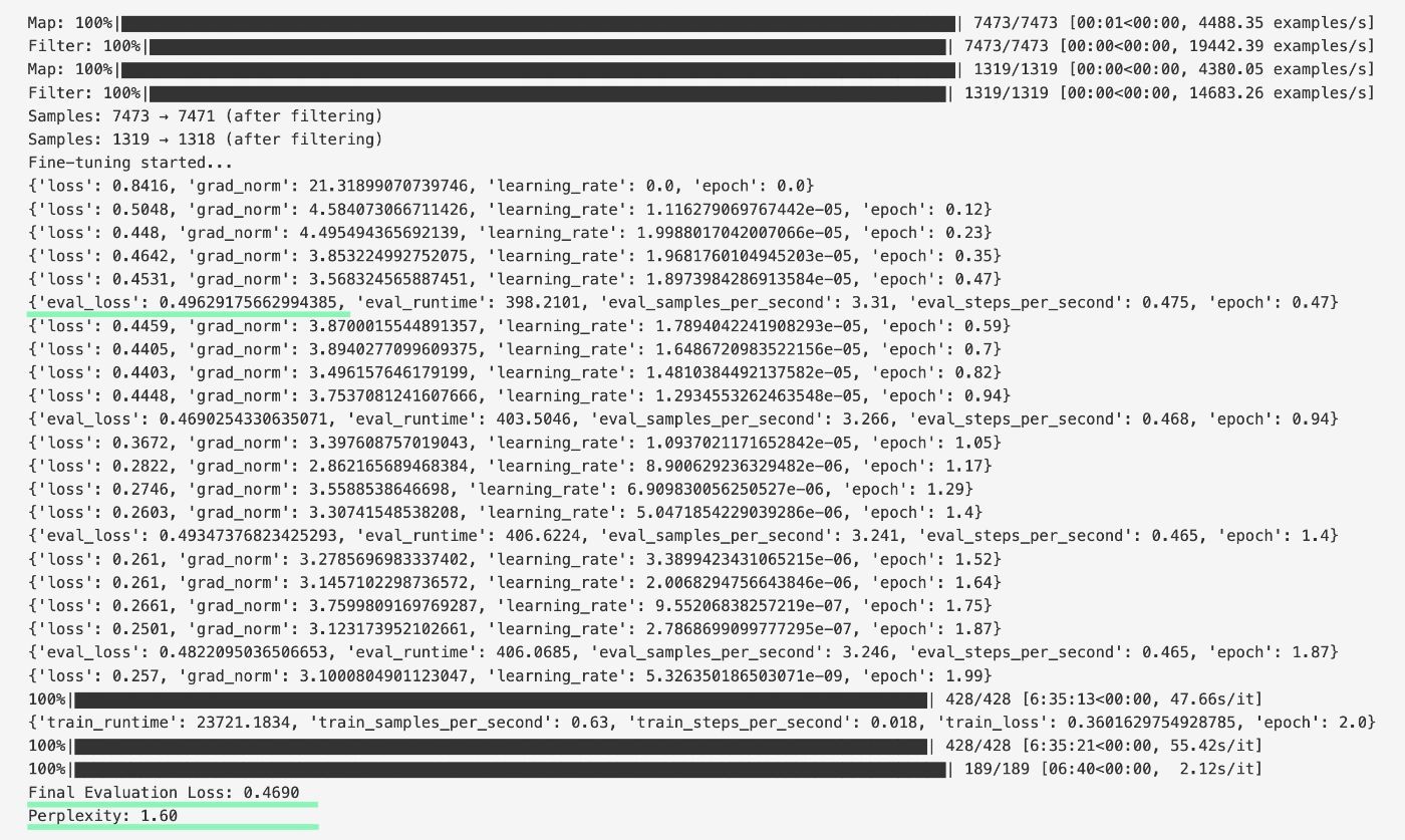
To give you a real-world reference, here’s what worked smoothly for us on a MacBook Air with the M4 chip and 16GB RAM. With this setup, it took around 6.5 hours to complete fine-tuning:
● Batch size for training: 7
● Batch size for eval: 7
● Gradient accumulation: 5
As your model trains, keep an eye on the evaluation loss. If it increases while training loss drops, the model is overfitting. In that case, adjust epochs, lower the learning rate, modify weight decay, and other hyperparameters. In the example below, we see healthy results with eval loss decreasing from 0.496 to 0.469 and a final perplexity of 1.60.
6. Test the Fine-Tuned Model
Now for the moment of truth – was our fine-tuning actually successful? You can manually test the fine-tuned model by prompting it with this Python code:
from transformers import pipeline

generator = pipeline(
    "text-generation",
    # Use `Qwen/Qwen2.5-0.5B` for testing the base model
    model="./qwen-math/final"
)

output = generator(
    "James has 5 apples. He buys 3 times as many. Then gives half away. How many does he have?",
    return_full_text=False
)
print(output[0]["generated_text"])
In this side-by-side comparison, you can see how the before and after models respond to the same question (the correct answer is 10):
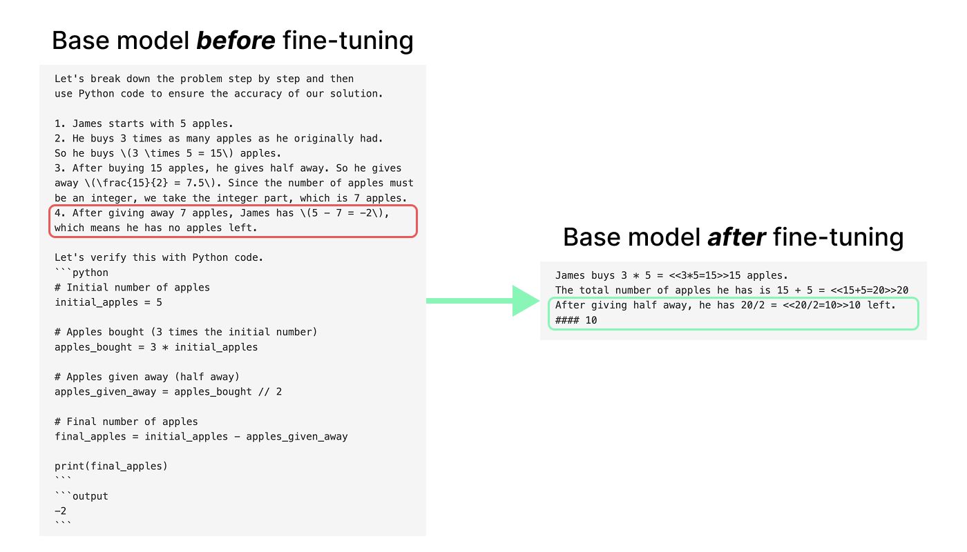
With sampling enabled, both models occasionally get it right or wrong due to randomness. But setting do_sample=False in the generator() function reveals their true confidence: the model always picks its highest-probability answer. The base model confidently outputs -2 (wrong), while the fine-tuned model confidently outputs 10 (correct). That’s the fine-tuning at work.
Fine-Tuning Best Practices
Model Selection
● Choose the right base model: Domain-specific models and appropriate context windows save you from fighting against the model’s existing knowledge.
● Understand the model architecture: Encoder-only models (like BERT) excel at classification tasks, decoder-only models (like GPT) at text generation, and encoder-decoder models (like T5) at transformation tasks like translation or summarization.
● Match your model’s input format: If your base model was trained with specific prompt templates, use the same format in fine-tuning. Mismatched formats confuse the model and tank performance.
Data Preparation
● Prioritize data quality over quantity: Clean and accurate examples beat massive and noisy datasets every time.
● Split training and evaluation samples: Never let your model see evaluation data during training. This lets you catch overfitting before it ruins your model.
● Establish a “golden set” for evaluation: Automated metrics like perplexity don’t tell you if the model actually follows instructions or just predicts words statistically.
Training Strategy
● Start with a lower learning rate: You’re making minor adjustments, not teaching it from scratch, so aggressive rates may erase what it learned during pre-training.
● Use parameter-efficient fine-tuning (LoRA/PEFT): Train only 1% of parameters to get 90%+ performance while using way less memory and time.
● Target all linear layers in LoRA: Targeting all layers (q_proj, k_proj, v_proj, o_proj, etc.) yields models that reason significantly better, not just mimic style.
● Use NEFTune (noisy embedding fine-tuning): Random noise in embeddings acts as regularization, which can prevent memorization and boost conversational quality by 35+ percentage points.
● After SFT, Run DPO: Don’t just stop after SFT. SFT teaches how to talk; DPO teaches what is good by learning from preference pairs.
What Are the Limitations of LLM Fine-Tuning?
● Catastrophic forgetting: Fine-tuning overwrites existing neural patterns, which can erase valuable general knowledge the model learned during pre-training. Multi-task learning, where you train on your specialized task alongside general examples, can help preserve broader capabilities.
● Overfitting on small datasets: The model may memorize your training examples instead of learning patterns, causing it to fail on slightly different inputs.
● High computational cost: Fine-tuning billions of parameters requires expensive GPUs, significant memory, and hours to days or weeks of training time.
● Bias amplification: Pre-trained models already carry biases from their training data, and fine-tuning can intensify these biases if your dataset isn’t carefully curated.
● Manual knowledge update: New and external knowledge may require retraining the entire model or implementing Retrieval-Augmented Generation (RAG), while repeated fine-tuning often degrades performance.
Conclusion
Fine-tuning works, but only if your data is clean and your hyperparameters are dialed in. Combine it with prompt engineering for the best results, where fine-tuning handles the task specialization while prompt engineering guides the model’s behavior at inference time.
Continue by grabbing a model from Hugging Face that fits your use case for domain-specific fine-tuning, scrape or build a quality dataset for your task, and run your first fine-tuning session on a small subset. Once you see promising results, scale up and experiment with LoRA, DPO, or NEFTune to squeeze out better performance. The gap between reading this tutorial and having a working specialized model is smaller than you think.