Essential Python Libraries for Data Science

digitado ⋅ 3 de March de 2026

Part 3: Classical Machine Learning

In Part 1, we focused on how data is represented, transformed, and computed using NumPy and Pandas. By the end of that part, the dataset was clean, structured, and numerically stable.

In Part 2, we resisted the urge to jump straight into modeling. Instead, we validated assumptions through visualization and diagnostics. We inspected distributions, examined feature relationships, identified correlation and redundancy, and documented constraints that would influence downstream decisions.

At this point, the data is not just prepared. It is understood.

Only now does it make sense to introduce machine learning.

This is an important distinction. Classical machine learning does not add intelligence to raw data. It formalizes patterns that already exist. When modeling is introduced too early, it amplifies noise, hidden bias, and data quality issues. When introduced at the right time, it becomes a powerful and reliable decision-making layer.

This third part continues in the same notebook, using the same normalized and diagnosed dataset from Parts 1 and part 2. No data is reloaded. No features are redefined. The diagnostic observations already recorded will now influence how models are built, evaluated, and interpreted.

The focus here is classical machine learning for structured, tabular data, using scikit-learn. Not from a competition perspective, and not as a catalog of algorithms, but as a systematic modeling process that prioritizes stability, interpretability, and reproducibility.

We will start with simple, well-understood baselines, build pipelines that reflect real workflows, and evaluate models in a way that aligns with production constraints rather than leaderboard metrics.

By the end of this part, you will not just have trained models. You will have a modeling approach that fits naturally into the data pipeline we have built so far.

In this part, we will:

Split data correctly while preserving assumptions
Build preprocessing and modeling pipelines
Train baseline models for structured data
Evaluate performance using appropriate metrics
Establish a foundation for more advanced models in later parts

Each step will extend the same end-to-end example, without resetting or reshaping the workflow.

Transition to Modeling

With data prepared in Part 1 and validated in Part 2, the next step is to introduce machine learning in the most conservative and reliable way possible.

We begin by defining how data flows into a model.

Step 11: Train–Test Split — Defining the Boundary Between Learning and Evaluation

Once data has been prepared and validated, the first modeling decision is not which algorithm to use. It is how to separate what the model is allowed to learn from what it will be evaluated on.

This boundary is critical. A poorly designed train–test split introduces leakage, inflates performance metrics, and creates false confidence that only collapses later in production. A well-designed split enforces discipline and makes model evaluation meaningful.

In real systems, models are always evaluated on future or unseen data. The train–test split is the simplest approximation of that reality.

Because the dataset we are working with is already normalized and diagnostically validated, this step is not about fixing data issues. It is about preserving assumptions and ensuring that evaluation reflects how the model will actually be used.

Why Train–Test Splitting Comes Before Modeling

Many beginners treat the train–test split as a mechanical step. In production environments, it is a design decision.

Key considerations include:

Preventing information leakage
Ensuring reproducibility
Maintaining alignment with downstream evaluation
Establishing a stable baseline for comparison

Once this split is defined, everything that follows must respect it.

Step 11.1: Defining Features and Target

We continue using the same feature set and target defined earlier. Nothing is reloaded and nothing is redefined.

X = X_normalized_df
y = df["target"]

At this stage:

X represents normalized numerical features
y represents the classification target
Both are already validated and aligned

Step 11.2: Performing the Train–Test Split

We now split the dataset into training and testing subsets. The test set represents unseen data and must remain untouched until evaluation.

from sklearn.model_selection import train_test_split

X_train, X_test, y_train, y_test = train_test_split(
    X,
    y,
    test_size=0.2,
    random_state=42,
    stratify=y
)

Key points about this split:

test_size=0.2 reserves 20% of data for evaluation
random_state=42 ensures reproducibility
stratify=y preserves class distribution, which is essential for classification problems

Stratification is particularly important in real-world datasets where class imbalance is common. Without it, evaluation metrics can become misleading.

What This Split Guarantees

At this point, we have enforced several important constraints:

The model will only learn from X_train and y_train
Evaluation will be performed only on X_test and y_test
No diagnostic or preprocessing logic will peek into the test set
Performance metrics will reflect generalization, not memorization

These guarantees are more important than the choice of algorithm that follows.

Why This Matters in Production Systems

In production, models rarely fail because they are mathematically incorrect. They fail because evaluation was optimistic, assumptions were violated, or leakage went unnoticed.

A clean train–test split is the first safeguard against these failures. It establishes trust in every metric computed afterward and provides a stable foundation for comparing models as the system evolves.

Transition to the Next Step

With the learning and evaluation boundary clearly defined, we can now introduce models in a controlled and interpretable way.

Step 12: Baseline Models — Establishing Reference Performance

Once the train–test boundary has been defined, the next step is not to search for the most powerful algorithm. It is to establish baselines.

Baseline models serve a specific purpose in production-grade data science. They answer a simple but critical question:

What level of performance can we achieve with the simplest, most interpretable assumptions?

Without baselines, improvements cannot be measured meaningfully. More complex models may appear to perform well, but without a reference point, it is impossible to know whether that performance is real or accidental.

In structured, tabular data problems, linear models are often the most informative place to start.

Why Baseline Models Matter

Baseline models provide several important guarantees:

They are fast to train and evaluate
Their behavior is easy to interpret
Their limitations are well understood
They expose data issues early
They create a stable benchmark for comparison

If a sophisticated model cannot significantly outperform a well-chosen baseline, the additional complexity is rarely justified.

Step 12.1: Logistic Regression as a Baseline Classifier

Because this is a binary classification problem, Logistic Regression is a natural starting point. Despite its simplicity, it performs surprisingly well on many real-world datasets and provides clear signals about feature relevance.

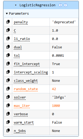
We will use scikit-learn’s implementation with default settings, keeping the model intentionally simple.

from sklearn.linear_model import LogisticRegression

log_reg = LogisticRegression(
    max_iter=1000,
    random_state=42
)
log_reg.fit(X_train, y_train)

At this stage:

The model is trained only on training data
No hyperparameter tuning is performed
The goal is reference performance, not optimization

Step 12.2: Evaluating the Baseline Model

Evaluation must be performed strictly on the test set. Any evaluation on training data would overstate performance and undermine the purpose of the baseline.

from sklearn.metrics import accuracy_score

y_pred = log_reg.predict(X_test)
accuracy = accuracy_score(y_test, y_pred)
accuracy

Accuracy provides a quick sanity check, but it should never be the only metric considered. It answers how often predictions are correct, not how or why they fail.

Step 12.3: Confusion Matrix for Error Structure

To understand model behavior more deeply, we examine the confusion matrix. This reveals the types of errors the model makes and whether those errors are symmetric.

from sklearn.metrics import confusion_matrix

conf_matrix = confusion_matrix(y_test, y_pred)
conf_matrix

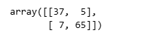
This matrix highlights:

False positives vs false negatives
Whether one class is systematically harder to predict
Potential business implications of misclassification

These patterns often matter more than raw accuracy.

Step 12.4: Classification Report for Detailed Metrics

Finally, we examine precision, recall, and F1-score to understand performance per class.

from sklearn.metrics import classification_report

print(classification_report(y_test, y_pred))

This report provides a more complete picture of model behavior and often exposes trade-offs hidden by aggregate metrics.

What This Baseline Tells Us

At this point, we have established a clear reference point:

Performance achieved with minimal assumptions
Error patterns that reflect data structure
A model that is easy to interpret and debug

This baseline becomes the yardstick against which all future models will be measured.

Why This Step Is Critical in Production

In production systems, baseline models are often retained even after more advanced models are deployed. They serve as:

Fallback options
Sanity checks during retraining
Reference points during model drift analysis

Skipping baselines removes this safety net.

Transition to the Next Step

With a baseline model in place, we can now focus on structure rather than algorithms.

In the next step, we will introduce scikit-learn pipelines to formalize preprocessing and modeling as a single, reproducible unit.

Step 13: Modeling Pipelines — Structuring Training and Evaluation

Once a baseline model is established, the next priority is not improving performance. It is improving structure.

In exploratory work, it is common to see preprocessing steps applied manually before model training. In production systems, this approach quickly becomes fragile. Transformations drift, evaluation becomes inconsistent, and retraining pipelines break in subtle ways.

Modeling pipelines exist to prevent this.

A pipeline enforces a single, repeatable path from raw input to prediction. Every transformation applied during training is guaranteed to be applied in the same way during evaluation and inference. This consistency is what turns a model into a system component rather than a one-off experiment.

Why Pipelines Matter More Than Algorithms

In real deployments, models fail far more often due to process issues than algorithmic limitations.

Pipelines address several recurring problems:

Inconsistent preprocessing between training and inference
Accidental leakage from test data
Difficulty reproducing results
Fragile retraining workflows

Once pipelines are in place, models become easier to reason about, easier to validate, and easier to operate over time.

Step 13.1: Introducing the scikit-learn Pipeline

scikit-learn provides a native Pipeline abstraction that allows preprocessing and modeling steps to be chained together into a single object.

Even when preprocessing is minimal, using a pipeline early establishes good discipline.

from sklearn.pipeline import Pipeline
from sklearn.linear_model import LogisticRegression

Step 13.2: Defining a Simple Modeling Pipeline

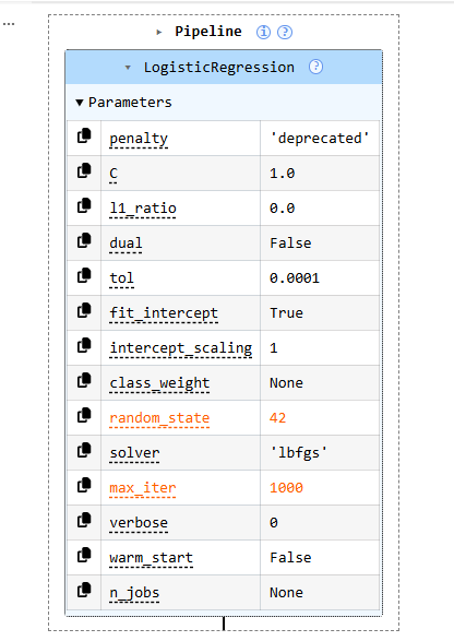
In our case, the data is already numerically normalized. That does not eliminate the need for a pipeline. It simply means the pipeline is currently lightweight.

pipeline = Pipeline(
    steps=[
        ("model", LogisticRegression(
            max_iter=1000,
            random_state=42
        ))
    ]
)

This pipeline explicitly defines:

A single modeling step
All model configuration in one place
A reusable object that encapsulates training logic

As the system evolves, additional steps can be added without changing downstream code.

Step 13.3: Training the Pipeline

Training the pipeline looks identical to training a model, but the semantics are different. The pipeline now owns the full transformation and modeling process.

pipeline.fit(X_train, y_train)

This single call ensures that:

All steps are fit only on training data
No accidental leakage occurs
The training process is reproducible

Step 13.4: Evaluating the Pipeline

Evaluation also remains unchanged at the surface level, which is a key advantage of pipelines.

y_pred_pipeline = pipeline.predict(X_test)

from sklearn.metrics import accuracy_score
accuracy_score(y_test, y_pred_pipeline)

Because the pipeline encapsulates all logic, the same object can later be used for inference without modification.

Step 13.5: Why Pipelines Scale Well

As systems grow, pipelines become even more valuable. They support:

Adding preprocessing steps safely
Swapping models without refactoring code
Cross-validation without leakage
Consistent retraining and deployment

In regulated or long-lived systems, pipelines are often a requirement rather than a convenience.

Pipelines as System Boundaries

A useful way to think about pipelines is as contract boundaries. Everything inside the pipeline is part of the learning system. Everything outside is orchestration.

This separation simplifies:

Auditing
Debugging
Monitoring
Change management

It also makes the system more resilient to future changes.

Transition to the Next Step

With pipelines in place, we can now evaluate models more rigorously and compare alternatives without changing process.

In the next step, we will focus on model evaluation beyond accuracy, examining metrics that reveal error structure and business impact.

Step 14: Model Evaluation — Metrics That Actually Matter

Once a model has been trained through a clean pipeline, the next question is not whether it achieves a high score, but what that score actually means.

In many projects, evaluation stops at a single metric, often accuracy. In production systems, this is rarely sufficient. A model can achieve high accuracy while still making costly or unacceptable errors. Evaluation must therefore expose error structure, not just aggregate performance.

This step focuses on understanding how the model fails, not just how often it succeeds.

Why Accuracy Alone Is Not Enough

Accuracy answers one question: What fraction of predictions were correct?

It does not answer:

Which class is harder to predict
Whether false positives or false negatives dominate
How performance varies across decision thresholds
Whether errors align with business risk

In regulated or high-impact systems, these distinctions matter more than raw accuracy.

Step 14.1: Reusing Pipeline Predictions

We continue evaluating the pipeline model introduced in Step 13. No new models are trained and no parameters are changed.

y_pred = pipeline.predict(X_test)

This ensures that evaluation reflects the exact system that would be deployed.

Step 14.2: Confusion Matrix — Understanding Error Types

The confusion matrix is one of the most important diagnostic tools in classification. It shows how predictions are distributed across true classes.

from sklearn.metrics import confusion_matrix

conf_matrix = confusion_matrix(y_test, y_pred)
conf_matrix

This matrix reveals:

How often the model confuses one class for another
Whether errors are balanced or skewed
Which mistakes are most common

In real systems, these patterns often map directly to business outcomes.

Step 14.3: Precision, Recall, and F1-Score

To go beyond raw counts, we examine class-level performance using precision, recall, and F1-score.

from sklearn.metrics import classification_report

print(classification_report(y_test, y_pred))

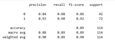
These metrics provide deeper insight:

Precision measures how reliable positive predictions are
Recall measures how well the model captures actual positives
F1-score balances the two

Different applications prioritize these metrics differently. Understanding the trade-offs is more important than optimizing any single value.

Step 14.4: Probability Scores and Decision Thresholds

Many models, including logistic regression, produce probability estimates rather than hard class labels. These probabilities allow decision thresholds to be adjusted based on risk tolerance.

y_proba = pipeline.predict_proba(X_test)[:, 1]

Working with probabilities enables:

Threshold tuning
Risk-based decisioning
Better alignment with business constraints

This is especially important when the cost of different error types is asymmetric.

Step 14.5: ROC Curve and AUC

The ROC curve visualizes the trade-off between true positive rate and false positive rate across thresholds.

from sklearn.metrics import roc_curve, roc_auc_score

fpr, tpr, thresholds = roc_curve(y_test, y_proba)
roc_auc = roc_auc_score(y_test, y_proba)
roc_auc

AUC provides a threshold-independent measure of separability. While it should not be used in isolation, it is useful for comparing models under consistent conditions.

Interpreting Evaluation Results in Context

Evaluation metrics do not exist in a vacuum. Their meaning depends on:

Data distribution
Class imbalance
Business risk
Regulatory constraints

A model that is statistically strong but operationally risky is not production-ready. Evaluation is where these tensions surface.

Why This Step Matters in Production

In production systems:

Metrics guide deployment decisions
Metrics define alert thresholds
Metrics drive retraining schedules
Metrics support audits and reviews

Poor evaluation leads to fragile systems, regardless of model sophistication.

Transition to the Next Step

At this point, we have:

A validated dataset
A reproducible pipeline
A baseline model
A meaningful evaluation framework

In the next step, we will bring these elements together and discuss model selection, comparison, and readiness for more advanced approaches, setting the stage for Part 4.

Step 15: Model Comparison and Readiness — Knowing When to Move Forward

By this point, we have done everything that classical machine learning requires to be credible.

We did not rush into complex algorithms. We built a clean data foundation, validated assumptions, enforced strict training boundaries, established baselines, structured the workflow with pipelines, and evaluated models using metrics that expose real behavior.

Now comes a decision that many projects get wrong: whether to move forward, and how.

Model comparison is not about picking the highest score. It is about deciding whether additional complexity is justified, safe, and aligned with system constraints.

What We Are Comparing Against

Our baseline model provides a reference point with several important properties:

It is interpretable
It is stable
It is fast to train and retrain
Its failure modes are easy to understand
Its performance is measurable and reproducible

Any model that follows must justify itself relative to this baseline, not in isolation.

When a Baseline Is “Good Enough”

In many real-world systems, baseline models remain in production for years. This is not a failure of ambition. It is a reflection of trade-offs.

A baseline may be sufficient when:

Performance meets business requirements
Errors are well understood and acceptable
Latency and throughput constraints are tight
Explainability is mandatory
Retraining and monitoring need to be simple

In these cases, complexity adds risk without meaningful upside.

When It Makes Sense to Go Further

More advanced models become relevant when:

Baseline performance is clearly insufficient
Error patterns indicate nonlinear structure
Feature interactions matter
Business impact justifies additional complexity
Monitoring and governance capabilities are in place

This decision should be driven by evidence, not by algorithm popularity.

Readiness Checklist Before Moving On

Before introducing more sophisticated models, the system should satisfy the following:

A stable baseline exists
Evaluation metrics are trusted
Error behavior is understood
Pipelines are in place
Retraining is reproducible
Monitoring requirements are clear

If any of these are missing, adding complexity will amplify existing weaknesses.

Why This Step Matters More Than Any Algorithm

Many production failures happen not because models are weak, but because teams move forward prematurely. They add complexity before establishing control.

This step enforces restraint.

It ensures that progress is deliberate and reversible, not reactive.

Closing Thoughts for Part 3

Classical machine learning is not outdated. It remains the backbone of most production systems built on structured, tabular data. What determines success is not the algorithm itself, but the process around it: disciplined data handling, careful evaluation, and awareness of real operational constraints.

By the end of this part, we have not simply trained models. We have established a modeling approach that is stable, interpretable, and designed to evolve safely as systems grow in complexity. This foundation is what allows teams to move forward with confidence rather than chasing incremental gains without control.

If this way of thinking reflects how you approach data science in real systems, consider clapping to signal that this perspective was useful, leaving a comment to share how you handle baselines and evaluation in your own work, or following the series to continue from classical modeling into more advanced production techniques. Sharing the article with others working on tabular ML systems also helps extend the discussion beyond a single post. Thanks !!!

Transition to Part 4

With a solid classical modeling foundation in place, we are now ready to explore gradient boosting in production.

In Part 4, we will examine why models such as XGBoost, LightGBM, and CatBoost dominate tabular machine learning, and how they are tuned, evaluated, and governed in real-world systems where performance, explainability, and stability all matter.

Essential Python Libraries for Data Science was originally published in Towards AI on Medium, where people are continuing the conversation by highlighting and responding to this story.

Like 0

Liked Liked