DELIVERY DELAY PREDICTOR: Machine Learning System for Logistics Optimization

This project was presented as the final project to obtain the Founderz AI Business School + Microsoft certificate in AI and Innovation 2025.

Summary

In contemporary logistics, punctuality has emerged as a fundamental pillar for customer loyalty and business competitiveness. However, a significant part of supply chains continue to operate under reactive paradigms, limiting themselves to managing delays only when they have already materialized.

This project addresses this inefficiency by developing a comprehensive solution (End-to-End) based on Artificial Intelligence, with the aim of anticipating the risk of delay at the precise moment of purchase. The technological proposal consists of the deployment of a Machine Learning model (Random Forest), operationalized through an interactive web application in Streamlit to facilitate decision-making in real time.

After an exhaustive cleaning and feature engineering process on the DataCo Supply Chain dataset, the model achieved an accuracy of 71.8% and an area under the curve (AUC) of 0.77 in the validation set. Beyond the technical metrics, the strategic value of the project lies in setting the decision threshold to 30%, a measure designed to prioritize the sensitivity (Recall) of the system. This calibration allows the vast majority of critical shipments to be identified, enabling operations managers to implement preventive actions and effectively transforming logistics management from a corrective model to an eminently predictive one.

1. INTRODUCTION

1.1. Context: Logistics as an engine of the Global Economy

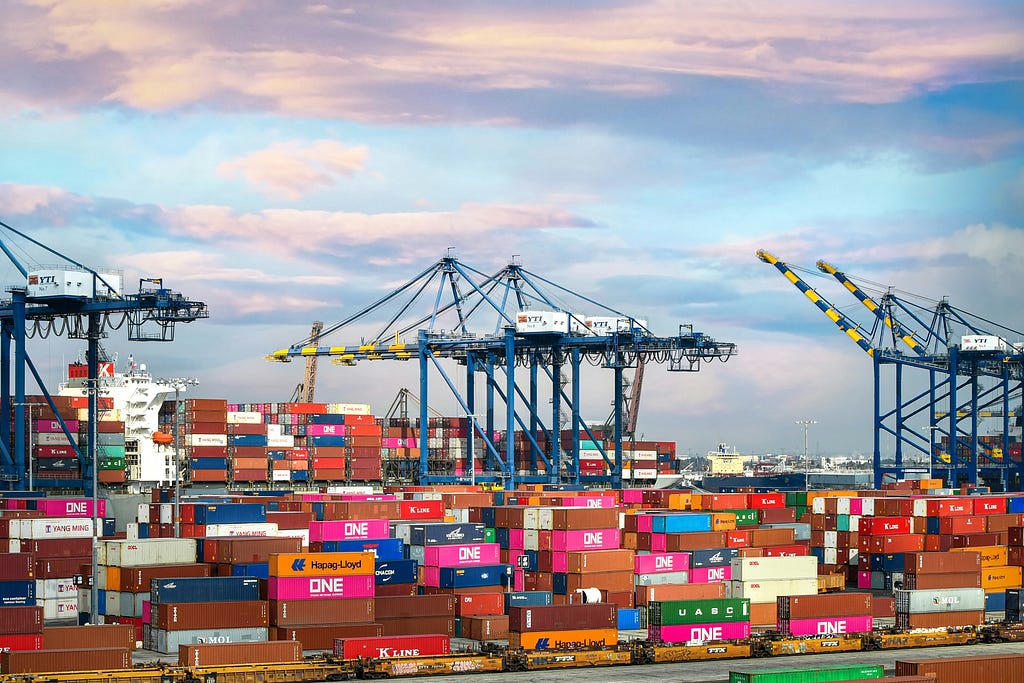
The last decade has witnessed an unprecedented transformation in the global trade ecosystem. The rise of e-commerce and the globalization of markets have redefined the role of logistics, which has ceased to be considered a mere center of operational costs to become a strategic pillar of competitive advantage. In this new scenario, the supply chain no longer just moves boxes; it manages expectations, experiences and, fundamentally, customer loyalty.

This paradigm shift is driven by what the industry calls the “Amazon Effect”: the standardization of increasingly shorter, accurate, and transparent delivery times. Today’s hyper-connected and demanding consumers have raised their service expectations to historic levels. According to recent studies in the logistics sector, tolerance for delay is practically zero; A failed shipment not only involves direct costs of return or compensation, but reputational damage that often results in the customer’s final loss (churn).

In parallel to this operational requirement, companies are experiencing the Industry 4.0 revolution. Modern supply chains generate massive amounts of data through ERP (Enterprise Resource Planning) systems, WMS (Warehouse Management Systems) and IoT devices. However, there is a significant paradox in the sector: organizations are “Data Rich, Information Poor”.

Traditionally, the analysis of this data has been limited to a descriptive approach: reports and dashboards explaining what happened yesterday (how many orders were delayed last month). While this is useful for accounting, it is insufficient for day-to-day operation in a volatile market. The complexity of the variables that affect a shipment (routes, modes of transport, customer geography, seasonality) is beyond the capacity of human analysis or conventional spreadsheet tools.

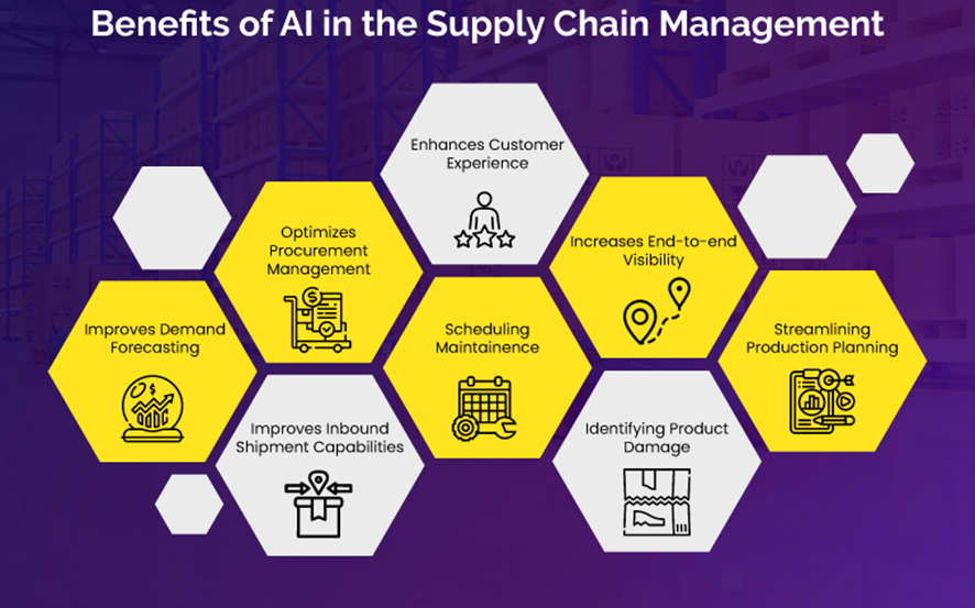
It is at this inflection point that Artificial Intelligence (AI) and Machine Learning (ML) emerge not as a futuristic option, but as an imperative necessity. The ability of algorithms to process large volumes of historical data, detect non-linear patterns and, most importantly, anticipate future scenarios, offers the opportunity to evolve towards a “Predictive Supply Chain”. This project is precisely in this context: to harness the latent asset of historical data to solve logistics’ oldest problem: delivery uncertainty.

1.2. Problem Statement

Despite the advances in digitalization described above, supply chain incident management suffers from a structural deficiency: reactivity. In the current operations of most logistics companies, the detection of a delay occurs simultaneously or after it materializes. This approach, which we could call “post-mortem management”, means that the operations manager only receives the alert when the truck has no longer arrived at its destination or, in the worst case, when the customer contacts the customer service to claim their order.

This inability to anticipate failure generates a cascade of inefficiencies that have a direct impact on the income statement:

1. Incremental Operational Costs: The resolution of hot incidents forces the use of emergency solutions (urgent replacement shipments, overtime of personnel), which are exponentially more expensive than standard planning.
2. Customer Lifetime Value (CLV) erosion: In a market where the competition is just a click away, reliability is the currency. An unreported delay not only affects a one-off sale, but also breaks trust, increasing the churn rate and making it difficult to attract new customers due to the deterioration of online reputation.
3. Data Asset Underutilization: Organizations store terabytes of historical data about their shipments (routes, times, product characteristics), but this data resides in “silos” or is used merely for past audits. There is no automated bridge that transforms the accumulated historical experience into preventive intelligence for future shipments.

The central problem that motivates this work, therefore, is not the lack of data, but the lack of actionable predictive capacity. Traditional systems (ERPs and spreadsheets) are deterministic and linear; They fail to capture the complexity and uncertainty of real logistics, where hidden variables (such as the correlation between a specific geographic region and a type of shipment) can be determinants.

Faced with this scenario, the research question that underpins this project arises:

Is it possible to develop an analytical model based on Machine Learning that, by learning from the historical patterns of the supply chain, allows predicting with greater reliability than chance the risk of delay of an order at the time of its creation, thus allowing preventive intervention instead of corrective intervention?

1.3. Motivation and Justification

The main motivation for the development of this project stems from the convergence between an unmet market need and current technological maturity. In an environment where logistics margins are increasingly narrow, the justification for this work is based on three fundamental pillars: economic impact, technological innovation and the democratisation of data.

1.3.1. Economic and Business Justification

Reactive delay management represents a massive “hidden cost” for organizations. The motivation of this system is to transform this cost center into a sustainable competitive advantage:

• Operating Margin Protection: By anticipating a delay, the company can take low-cost measures (such as notifying the customer or prioritizing warehouse processing) instead of high-cost measures (urgent replenishment shipments or subsequent financial compensation).
• Loyalty and Customer Lifetime Value (LTV): Transparency is now more valued than speed. A customer who is proactively alerted to a delay (“Your order will arrive on Thursday instead of Tuesday”) maintains a higher level of satisfaction than who discovers the delay on their own. This project seeks to reduce the churn rate (abandonment) through data-driven expectation management.

1.3.2. Technical and Scientific Justification

From a technical point of view, this work is justified by the need to overcome the limitations of traditional heuristic systems. Conventional tools usually base their estimates on simple rules (e.g.: “If the distance is > 500km, it takes 3 days”).

This project demonstrates that the application of Machine Learning algorithms (specifically Random Forest) provides superior value because:

1. Captures Non-Linearity: It is able to detect complex patterns that escape human intuition (e.g., how the “payment type” interacts with the “sending region” to increase the risk of delay).
2. Continuous Learning: Unlike static software, the proposed model has the ability to retrain and adapt to new patterns of market behavior, offering a scalable and resilient solution.

1.3.3. Social and Operational Justification (Democratization of AI)

Finally, a critical motivation of this TFM is to bridge the gap between data science and day-to-day operation. Powerful predictive models are often locked into code environments (Python notebooks) that are inaccessible to business personnel.

The implementation of the interface in Streamlit justifies the project as an operational empowerment tool: it allows a warehouse manager or customer service agent, without programming knowledge, to use advanced artificial intelligence to make informed decisions in real time. This transforms AI from an abstract “black box” to a tangible and useful work tool.

1.4. Objectives

The fundamental purpose of this Master’s Thesis is to demonstrate how technology can solve a tangible business problem by implementing a complete Artificial Intelligence solution.

1.4.1. General Objective

Design, develop and implement a comprehensive solution (End-to-End) based on Supervised Learning algorithms for the probabilistic prediction of delays in the supply chain.

1.4.2. Specific Objectives

In order to achieve the general objective, the following technical and functional goals have been established:

1. Data Engineering and Quality: Perform an exhaustive Exploratory Data Analysis (EDA) on the DataCo Supply Chain dataset, executing a rigorous cleaning and transformation process.
2. Model Development and Selection: Train, evaluate, and compare different classification algorithms. Select and optimize the model, justifying its choice based on performance metrics.
3. Strategic Business Alignance: Define and calibrate a custom decision threshold, prioritizing the Recall metric over pure Accuracy. The goal is to minimize False Negatives to ensure that the system alerts on the vast majority of problematic shipments.
4. Operationalization (Deployment): Develop a functional web application using the Streamlit framework, which serves as a user interface (Front-End). This tool should allow the visualization of KPIs in real time and the simulation of new shipments.

1.5. Project Limitations

Although the present work meets the objectives of developing a functional prototype, it is necessary to establish the following limitations inherent to the academic scope and available resources:

1. Static Data Character: The model has been trained and validated using a static historical data set (snapshot). In a real production environment, the solution would require an MLOps architecture for continuous retraining that mitigates model degradation (data drift) over time.
2. Absence of Real-Time Integration: The developed application operates as a standalone module. The bidirectional connection via API with corporate management systems (ERP or WMS) has not been implemented, so the ingestion of data for prediction requires, in this phase, a manual load or simulation.
3. Exogenous Variables Not Considered: The algorithm bases its predictions on endogenous variables of the order (customer, product, route). External real-time data sources that influence logistics, such as adverse weather conditions, road traffic, or unforeseen geopolitical situations, have not been integrated.
4. Local Computing Infrastructure: The data processing and execution of the model have been carried out in a local environment. For a large-scale deployment with millions of daily transactions, migration to a distributed cloud computing architecture (e.g., Azure Databricks or AWS SageMaker) would be necessary.

2. THEORETICAL FRAMEWORK

2.1. Logistics 4.0 and the Smart Supply Chain

The concept of Logistics 4.0 arises from the application of Industry 4.0 technologies: such as the Internet of Things (IoT), Cloud Computing and Big Data, to Supply Chain Management. This transformation redefines the logistics paradigm: the focus is no longer solely on the efficient physical movement of goods but on the intelligent management of the flow of information.

According to McKinsey & Company (2016), the transition to a digital and interconnected supply chain can reduce operating costs by up to 30% and reduce lost inventory by 75%. Unlike the traditional linear and fragmented model, Logistics 4.0 operates as an integrated ecosystem where visibility is total and in real time.

However, mere digitalization has generated a paradox in the sector: companies are “Data Rich, Information Poor”. Although they have terabytes of historical records thanks to ERP systems and sensors, many organizations lack the analytical capacity to transform that data into strategic decisions, limiting themselves to reactive management instead of taking advantage of the predictive potential of their digital assets.

2.2. Artificial Intelligence: From the Descriptive to the Predictive

This project is located in the evolutionary stage of Predictive Analytics. Unlike traditional systems based on hard-coded rules, which operate under static logic (e.g., “If distance > 500km, then time = 3 days”), predictive analytics uses machine learning algorithms to model uncertainty.

The superiority of this approach in supply chain management lies in its ability to handle non-linearity and the complex interaction between variables. A supervised learning algorithm does not assume predefined rules, but infers probabilistic patterns from historical data.

This allows you to identify subtle correlations such as the combined impact of payment method, geographic region, and product category to calculate the likelihood of a delay before the shipment leaves the warehouse, transforming operations management from a corrective to a preventive approach.

2.3. Ranking Algorithms and Random Forest Selection

From a Machine Learning perspective, predicting whether an order will be late or on time is formulated as a supervised binary classification problem. The goal is to train a mathematical function capable of assigning a discrete label on an input feature vector ().

Although the literature offers various algorithms for this purpose such as Logistic Regression, Support Vector Machines (SVM) or Neural Networks, this project has selected the Random Forest Classifier algorithm as the ideal predictive engine.

2.3.1. Technical Fundamentals of the Algorithm

Random Forest (Breiman, 2001) is an “Ensemble Learning” method based on the Bootstrap Aggregating technique. Its operation consists of building a multitude of decision trees during training and generating as a result the class that is the mode (the majority vote) of the classes predicted by the individual trees.

Mathematically, if we consider a set of trees, the final prediction for a new instance is obtained by majority voting:

2.3.2. Justification of the Selection

Random Forest’s superiority for this specific use case is underpinned by three pillars:

1. Robustness vs. Overfitting: By averaging hundreds of decoupled trees, Random Forest reduces variance without increasing bias, generalizing better to new unknown orders.
2. Managing Nonlinear Relationships: The causes of a logistical delay are rarely linear. Factors such as “Shipping Region” interact in complex ways with “Shipment Type”.
3. Feature Importance: Random Forest allows the importance of each variable to be quantified by reducing impurity (Gini).

2.4. Deployment and Operationalization Technologies

The operationalization of an Artificial Intelligence model (commonly referred to as Deployment) is the critical phase where the mathematical algorithm is transformed into a usable software tool.

For the development of this project, a technological ecosystem based on Python has been selected, prioritizing flexibility, scalability and prototyping speed.

2.4.1. Python as an Analytical Engine

Python has established itself as the de facto standard in data science and machine learning.

• Pandas and NumPy: Used for efficient manipulation of tabular data structures and high-performance matrix calculation.
• Scikit-Learn: The base library for the implementation of the Random Forest algorithm, validation metrics and preprocessing.

2.4.2. Streamlit: User Interface for Data Science

Streamlit is an open-source framework that allows you to turn data scripts into pure interactive web applications. Its reactive architecture makes it easy to create an Interactive Dashboard where business users can:

1. Enter parameters for new orders using intuitive forms.
2. Visualize the probability of risk in real time.
3. Interpret the results using dynamic graphs (integrated with the Plotly library).

This technological choice democratizes access to AI, bridging the gap between code complexity and end-user need for simplicity.

3. METHODOLOGY AND DATA ANALYSIS

The success of any Artificial Intelligence model depends more on the quality of the data than on the complexity of the algorithm. This chapter details the methodological workflow applied, from the acquisition of the raw material (the dataset) to its transformation into a clean and bias-free training set.

3.1. Description of the Dataset

For the execution of this project, the DataCo Global Supply Chain Dataset has been selected, a publicly accessible dataset that has established itself as an academic standard for the analysis of logistics operations and Big Data.

3.1.1. Origin and Nature of Data

The dataset collects real transactional information (anonymized) that combines three critical dimensions of the business: Sales, Logistics and Finance. Unlike synthetic datasets, this file has the inherent imperfections and complexity of the real world, making it an ideal candidate for training robust machine learning models.

The volume of data amounts to approximately 180,000 transactional records. Each row in the dataset represents an item within a purchase order, providing a fine granularity that allows behavior to be analyzed not only by order, but by specific product.

3.1.2. Dictionary of Variables (Main Characteristics)

The original structure of the dataset stands out for its high dimensionality (more than 50 columns). For the purposes of this study, the variables have been categorized into four functional groups:

1. Temporal and Logistic Variables: They are the core of the predictive model. They include order and shipping dates, as well as modes of transport (Standard Class, First Class, Second Class, Same Day, etc…).
2. Geographical Variables: Detailed information on the topology of the supply network. It includes both the origin (country/city of the warehouse) and the destination of the customer (Order Country, Order Region, Order City, etc…).
3. Product and Business Variables: Attributes that describe what is moving. It includes Category Name (Electronics, Sports, etc.), product price and customer segment (Consumer, Corporate, Home Office).
4. Target Variable: The dataset includes the Late_delivery_risk field, a binary variable:

• 0: Shipment on time.
• 1: Delayed shipment.

3.2. Exploratory Data Analysis (EDA)

Exploratory Data Analysis (EDA) is the critical phase of understanding the problem. Before submitting the information to any algorithm, a descriptive and visual statistical study was carried out on the 180,519 records that make up the dataset, with the aim of identifying patterns, anomalies and determining factors of the delay.

The following are the four main findings that defined the post-modeling strategy.

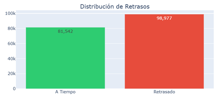
3.2.1. Balance of Classes and Dataset Health

The first step was to evaluate the distribution of the target variable (Late_delivery_risk). A severe imbalance would have required synthetic resampling techniques, but the analysis revealed a favorable scenario for machine learning:

• Global Delay Rate: 54.8% of registered orders suffered some type of delay.
• Conclusion: The dataset is considered technically balanced (close to 50/50 ratio). This validates the use of the Accuracy metric as a reliable indicator and eliminates the need to apply oversampling techniques (such as SMOTE) in the pre-processing phase.

3.2.2. Temporal Impact: The “Lag Gap”

The Days_Difference variable (difference between the scheduled date and the actual delivery date) was analyzed to quantify the operational impact. The results show a significant divergence:

• Delayed Shipments: They present an average deviation of +1.62 days from the promised date.
• On-Time Shipments: They arrive with an average advance of -0.71 days.
• Real Impact: In terms of customer experience, a delay is not just a binary breach, but adds an additional 2.33 days of average wait compared to a successful shipment.

3.2.3. Analysis by Mode of Submission: The “First Class” Paradox

One of the most counterintuitive and revealing findings of the study came from segmenting risk by shipping mode. Contrary to business logic, the most expensive service is the one with the highest risk of failure:

• First Class: Showed a critical delay rate of 95.3%.
• Standard Class: In contrast, the standard service turned out to be the most reliable, with a delay rate of only 38.1%.

This apparently contradictory phenomenon finds its justification in the theory of operational variability management. According to Christopher (2016), the reliability of a logistics system depends on its ability to absorb uncertainty through time margins.

The analysis suggests that the First Class mode operates with such tight delivery windows (low clearance) that it lacks the resilience to absorb the natural stochastic deviations of transport. Any minor incident, which in Standard mode would be absorbed by the safety margin of the delivery promise, results here in an immediate delay penalty.

3.2.4. Geographical Factors

The geographic analysis made it possible to identify “hot spots” in the global supply chain. Of the 23 regions analyzed, Central Africa stood out as the most problematic, with an incidence rate of 58.0%, suggesting local logistical complexities that the model must learn to penalize.

3.3. Preprocessing and Cleansing: Ensuring Data Integrity

The quality of a predictive model is intrinsically linked to the quality of the data that feeds it. After the exploratory analysis, a rigorous preprocessing phase was executed to transform the original dataset into a numerical matrix suitable for the training of the Random Forest algorithm.

This stage was structured in three fundamental interventions: the prevention of information leakage, the coding of variables and the elimination of noise.

3.3.1. Prevention of “Data Leakage”

The most important methodological challenge of this project was to guarantee the temporal honesty of the prediction. The original dataset contains variables that report a posteriori on the result of the shipment. Including these variables in training would have generated artificially perfect metrics (leak overfitting), but a useless model in reality.

Following a strict criterion of temporal causality, the following “cheating” variables were eliminated:

• Delivery Status: This variable explicitly indicates whether the shipment was “Late” or “Advance”.
• Days for shipping (real): This is the ex-post data of how long the shipment took.

By eliminating these columns, you ensure that the model only learns from the information available at the moment (order creation).

3.3.2. Encoding of Categorical Variables (Encoding)

The Random Forest algorithm requires numerical inputs. Since the dataset contains multiple categorical variables with high cardinality (many unique categories), such as Order Region or Category Name, the use of One-Hot Encoding was ruled out to avoid a dimensional explosion that would slow down the computation.

Instead, the Label Encoding technique was applied, transforming each category into a unique integer (e.g.: ‘Western Europe’ = 12, ‘South America’ = 34).

3.3.3. Noise Cleaning and Identifiers

Finally, those variables that do not provide predictive value or that introduce unique identifier bias were filtered:

• Personal Data: Customer Name, Customer Email, Customer Password. They were removed due to statistical irrelevance and privacy and data protection principles.
• Images: Columns such as Product Image that contained URLs.
• System Identifiers: Order ID, Customer ID. These numbers are correlative and not causal; including them could cause the model to memorize specific IDs instead of learning general patterns.

3.4. Variable Selection and Feature Engineering

Once the dataset had been cleaned, the next step was to identify which variables provide the greatest predictive power to the model. Unlike deep neural networks, which often operate as “black boxes,” the Random Forest algorithm offers an intrinsic advantage: the ability to calculate Feature Importance.

This calculation is based on the average decrease in impurity (Gini Impurity). In simple terms, the algorithm quantifies how much each variable contributes to “cleaning up” the decision and correctly separating delayed orders from one-off ones.

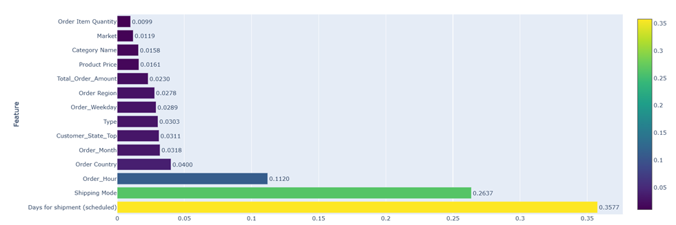
3.4.1. Ranking of Key Predictors

The importance analysis yielded a clear hierarchy on the risk factors in the supply chain. The variables that dominate the prediction, and therefore constitute the core of the model, are:

1. Days for shipping (scheduled): This is the strongest predictor. This is logical: the more aggressive the delivery promise (e.g., “same day” vs. “4 days”), the lower the margin of operational error and the greater the risk of default.
2. Order Region / City: Geography plays a determining role. As observed in the EDA, certain regions (such as Central Africa) have systemic infrastructure problems that the model has learned to penalize.
3. Shipping Mode: The shipping mode interacts directly with the scheduled days. The model detected that Premium ( First Class) modalities have a disproportionate failure rate.
4. Category Name: The type of product also plays a role (probably due to sizes, specific customs processes for certain goods, or suppliers associated with that category).

3.4.2. Reduction of Implied Dimensionality

This analysis confirmed that variables such as Payment Method or Customer Segment (Consumer vs. Corporate), although maintained in training, have a marginal impact on the prediction of logistics delay. This validates the hypothesis that the delay is primarily an operational and geographical problem, rather than a financial one.

The end result is an optimized dataset (X_train) that preserves only the strong signals, eliminating noise that could confuse the model and ensuring faster execution in the web application.

4. MODEL CONSTRUCTION AND OPTIMIZATION

4.1. Experimental Design and Overfitting Control

To guarantee the scientific validity of the model and ensure its generalizability in the face of new data, a rigorous evaluation protocol based on data partitioning was established.

4.1.1. Train-Test Split

A stratified random division of the processed dataset was applied, using the Scikit-Learn library:

• Training Set (80%): Used for the algorithm to learn the underlying patterns.
• Test Set (20%): Kept totally isolated (“invisible” to the model) during the training phase. This set acts as an impartial auditor to measure actual performance.

To ensure the reproducibility of the experiment, a random seed (random_state = 42) was set, ensuring that any future audit would obtain exactly the same distribution of data.

4.1.2. Verification of Absence of Overfitting

One of the main risks in tree-based algorithms is overfitting (memorizing the noise of training data). To rule out this phenomenon, performance metrics were compared between the two sets:

• Performance in Train: The model reached metrics close to 100% (expected behavior in Random Forest due to its depth).
• Test Performance: The model maintained a solid Accuracy of 71.8% and an AUC of 0.77 on unseen data.

Conclusion: The gap between training and test performance remains stable and within acceptable ranges for stochastic data of high human variability. The model has not memorized the data, but has learned generalizable patterns, validating its robustness.

4.2. Model Architecture and Configuration

The predictive core of the system is based on the Random Forest Classifier algorithm. This choice responds to its ability to handle mixed variables and capture nonlinear relationships without the need for scalar normalization.

The following configuration hyperparameters were set:

• n_estimators = 100: A “forest” of 100 decision trees was defined. This value represents the optimal equilibrium point (elbow point); Increasing the number of trees would increase computational cost without significantly improving predictive accuracy.
• criterion = ‘gini’: Gini impurity was used to measure the quality of divisions at each node of the tree.
• random_state = 42: Set to ensure deterministic and consistent results in each execution.
• n_jobs = -1: Configuration to use all available processor cores, optimizing training time through parallelization.

4.3. Threshold Tuning

One of the technical decisions with the greatest impact on the business was the modification of the classification threshold.

By default, binary classification algorithms assign the positive class (Delay) when the calculated probability is greater than 50% (0.5). However, in supply chain risk management, the costs of errors are not symmetrical:

• False Negative (High Cost): The model says it will be on time, but it is late. The customer gets frustrated, complains and reputations are damaged.
• False Positive (Low Cost): The model warns of a risk of delay that does not finally occur. Preventive action (notifying the warehouse) is low-cost.

4.3.1. Implementation of the Conservative Threshold (30%)

To align the model with the “maximum precaution” strategy, it was decided to reduce the Threshold from 0.5 standard to 0.30.

This means that if the model detects a delay probability greater than 30%, the system will automatically classify the shipment as “High Risk”.

Business Justification: This calibration prioritizes the Sensitivity (Recall) metric over Accuracy. We’d rather err on the side of caution and get a few false alarms in exchange for capturing the vast majority of real delays and protecting the customer experience.

5. RESULTS AND DISCUSSION

In this chapter, the results obtained after training the Random Forest model are presented and analyzed. The evaluation is not limited to pure statistical metrics, but delves into the operational interpretation of errors (Confusion Matrix) and the business impact derived from the adjustment of the decision threshold.

5.1. Evaluation of Model Performance

The model was evaluated using the Test Set (20%), ensuring that the metrics reflect the real ability to generalize to unseen data.

5.1.1. Global Metrics

The overall performance of the system is summarized in the following key indicators:

• Accuracy: The model correctly classified 71.8% of shipments. In a stochastic logistics context, where multiple human and external factors intervene, exceeding the 70% barrier is considered a robust and commercially viable result.
• ROC — AUC (Area Under the Curve): A value of 0.77 was obtained. This metric indicates that the model has a good discriminating capacity; that is, it has a 77% chance of scoring a “Real Delay” case higher than a randomly chosen “No Delay” case.

Illustration 11: Results: ROC

5.2. Analysis of the Confusion Matrix and the Operating Threshold

To understand where the model fails, it is necessary to decompose the errors through the Confusion Matrix, comparing the standard behavior (Threshold 0.5) against the proposed conservative strategy (Threshold 0.3).

5.2.1. The Accuracy vs. Sensitivity Dilemma (Recall)

In last-mile logistics, mistakes don’t cost the same:

• Type I Error (False Positive): The model predicts delay, but arrives on time. Cost: Low (an unnecessary preventive alert).
• Type II Error (False Negative): The model says “all right”, but the package arrives late. Cost: Very High (angry customer, complaint, possible loss of customer).

5.2.2. Impact of the Threshold Change to 30%

By moving the decision threshold to 0.30, the model is forced to be “hypersensitive” to risk.

• Result: A significant increase in Recall is observed. This means that the system is able to detect the vast majority of delays.
• Counterpart: False Positives Increase. However, from a business point of view, it is preferable to manage a proactive “false alarm”.

Illustration 12: Results — Simulation Parameters

5.3. Discussion of the Business Impact

The implementation of this predictive model offers a tangible competitive advantage over traditional reactive management:

1. Transition to Proactivity: Currently, companies react when the delay has already occurred. With this model, the intervention occurs at the time of purchase.
2. Expectation Management: By identifying risky shipments (e.g., First Class to Central Africa) with high probability, the company can adjust the promised date at checkout or proactively communicate to the customer, transforming a potential complaint into a transparent experience.
3. Prioritization of Resources: The warehouse cannot treat all orders as “urgent”. The risk score allows filtering and prioritizing only the 30–40% of orders that the model labels as critical, optimizing the effort of the staff.

5.4. Functional Validation: Implementation in Streamlit

To operationalize the mathematical model and allow its use by non-technical profiles (operations managers or Customer Service agents), an interactive web interface was developed using the Streamlit framework. This tool acts as the presentation layer that transforms the algorithm’s probabilities into business decisions.

The functional validation was divided into three components: navigation and metrics, historical intelligence visualization, and real-time predictive simulation.

5.4.1. Navigation and Control Panel

The application architecture was designed to be intuitive. As can be seen in the navigation sidebar, the user has immediate access to the system’s Quick Statistics.

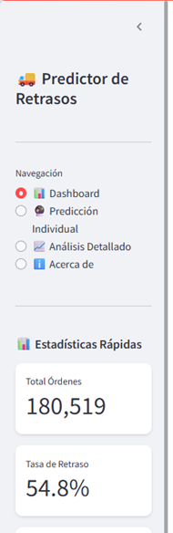
5.4.2. Business Intelligence Module

The first functional module provides a macroscopic view of the state of the supply chain. Its purpose is to enable the manager to identify systemic patterns before making individual predictions.

The dashboard integrates the critical visualizations derived from the analysis phase (EDA), highlighting:

1. Important Factors: Confirming that “Scheduled Days” and “Shipping Mode” are the main drivers.
2. Geographic Hot Spots: Identifying regions such as Central Africa or Southeast Asia as areas of high operational risk.

5.4.3. Individual Prediction Module (Simulator)

The operational core of the solution is the risk calculator. This interface allows you to enter the parameters of a new order before it is processed in the ERP. This is manual, but in an automated SC we should have it integrated once the purchase arrives.

The Input Form has been designed to capture the variables that the model requires:

5.4. Use Case Simulation: Critical Risk Detection

To validate the reliability of the tool in an operational environment, a full simulation was run within the Streamlit interface. The objective of this test was to verify if the model is capable of detecting a logistical incongruity (promising fast delivery on a slow route) and triggering the corresponding business alerts.

5.4.1. Scenario Configuration (Inputs)

In the control panel of the application, the parameters of a hypothetical order with high-risk characteristics (Stress Test) were entered:

• Destination Region: Southeast Asia , an area that historically has variable transit times.
• Shipping Method: Second Class. This is an inexpensive and generally time-consuming method.
• Scheduled days: 2 days (very ambitious).
• Product Category: Electronics (complex category, many delays=

Problem statement: We are trying to send a package to a distant region, using a slow transport method (Second Class), but promising the customer that it will arrive in only 2 days. Logically, this should be impossible.

5.4.2. Result Obtained in the Interface

The system processed the variables and returned the following visual response on the scorecard:

1. Calculated Probability: 81.09%.
2. Traffic Light Status: RED (HIGH RISK).
3. Action Message: “Attention: The probability exceeds the safety threshold (30%). Manual intervention is recommended.”

5.4.3. Interpretation and Validation of Logic

The result obtained makes full operational sense and validates the reasoning capacity of the model:

• Inconsistency Detected: The algorithm has detected the contradiction between the shipping method (Second Class, which usually takes 4–5 days) and the commercial promise (2 days).
• Geographical Weight: The Southeast Asia variable penalizes the prediction due to the logistical complexity of the region.
• Threshold operation: By obtaining 81.09%, the system has far exceeded the conservative threshold defined in the project (30%), correctly activating the alert protocol.

6. Conclusions and Future Lines

This Master’s Thesis has addressed the problem of uncertainty in the global supply chain through the development of a comprehensive Artificial Intelligence solution. Through the application of the Random Forest algorithm and its subsequent operationalization in a web interface, the hypothesis that logistical delays are not purely stochastic events, but predictable and manageable patterns, has been validated.

The main findings from the research and the proposed roadmap for the future evolution of the system are set out below.

6.1. Conclusions

After completing the project lifecycle, from data ingestion to application deployment, four key conclusions have been reached:

1. Technical Feasibility of the Predictive Model: It has been shown that it is possible to anticipate the risk of delay with an accuracy of 71.8% and an AUC of 0.77, using only information available at the time of purchase. This confirms that variables such as “Destination Region” and “Shipping Mode” contain enough signal to overcome traditional reactive management.
2. Methodological Rigor and “Data Leakage”: One of the pillars of the study has been the guarantee of temporal honesty. The identification and elimination of variables that leaked information from the future (such as Delivery Status or Days for actual shipping) ensures that the model is robust and applicable in a real production environment, avoiding the artificially inflated metrics that often affect theoretical projects.
3. Strategic Alignment (The 30% Threshold): The decision to adjust the decision threshold from the standard 50% to 30% has transformed the algorithm into a customer protection tool. While this configuration increases the false positive rate, it maximizes Recall, ensuring that the operation detects the vast majority of potential problems before they impact end-user satisfaction. Caution is prioritized over pure accuracy.
4. Democratization through Operationalization: The development of the application in Streamlit has bridged the gap between data science and logistics operation. It has been possible to turn a complex code into an intuitive interface that allows non-technical users (managers, support agents) to make decisions based on data in real time, validating the practical usefulness of the TFM.

6.2. Future Lines

While the current prototype meets the requirements of a Minimum Viable Product (MVP), three key areas have been identified for its evolution to a scalable enterprise solution:

• Integration via API (Microservices): The next logical step is to decouple the model from the visual interface and deploy it as a REST API (using FastAPI). This would allow the prediction to be integrated directly into the e-commerce checkout or ERP (SAP/Salesforce), automating the delivery promise without human intervention.
• Exogenous Data Enrichment: The current model uses endogenous data (company history). Accuracy could be significantly increased by incorporating external real-time data sources, such as weather forecasts on critical routes, port traffic status, or socio-political alerts in destination countries.
• MLOps Implementation and Retraining: Logistics are dynamic; routes change and new seasonal patterns emerge. To avoid model degradation (Data Drift), it is necessary to establish an MLOps pipeline that monitors performance and retrains the algorithm automatically with the latest data month by month.

---

DELIVERY DELAY PREDICTOR: Machine Learning System for Logistics Optimization was originally published in Towards AI on Medium, where people are continuing the conversation by highlighting and responding to this story.