DeepSeek-V3 from Scratch: Mixture of Experts (MoE)

---

---

DeepSeek-V3 from Scratch: Mixture of Experts (MoE)

In the first two parts of this series, we established the foundations of DeepSeek-V3 by implementing its core configuration and positional encoding, followed by a deep dive into Multi-Head Latent Attention (MLA). Together, these components set the stage for a model that is both efficient and capable of handling long-range dependencies. With those building blocks in place, we now explore another key innovation in DeepSeek-V3: the Mixture of Experts (MoE).

MoE introduces a dynamic way of scaling model capacity without proportionally increasing computational cost. Instead of activating every parameter for every input, the model selectively routes tokens through specialized “expert” networks, allowing it to expand representational power while keeping inference efficient. In this lesson, we’ll unpack the theory behind MoE, explain how expert routing works, and then implement it step by step. This installment continues our broader goal of reconstructing DeepSeek-V3 from scratch — showing how each innovation, from RoPE to MLA to MoE, fits together into a cohesive architecture that balances scale, efficiency, and performance.

This lesson is the 3rd in a 6-part series on Building DeepSeek-V3 from Scratch:

1. DeepSeek-V3 Model: Theory, Config, and Rotary Positional Embeddings
2. Build DeepSeek-V3: Multi-Head Latent Attention (MLA) Architecture
3. DeepSeek-V3 from Scratch: Mixture of Experts (MoE) (this tutorial)
4. Lesson 4
5. Lesson 5
6. Lesson 6

To learn about DeepSeek-V3 and build it from scratch, just keep reading.

---

The Scaling Challenge in Neural Networks

As we scale neural networks, we face a fundamental tradeoff: larger models have greater capacity to learn complex patterns, but they’re more expensive to train and deploy. A standard Transformer feedforward layer applies the same computation to every token:

,

where and are weight matrices, typically with . For our model with , this means , giving us approximately 256K parameters per FFN (FeedForward Network) per layer.

To increase model capacity, we could simply make larger — say, instead of . This doubles the FFN parameters and theoretically doubles capacity. But it also doubles the computation for every token, even if most don’t need that extra capacity.

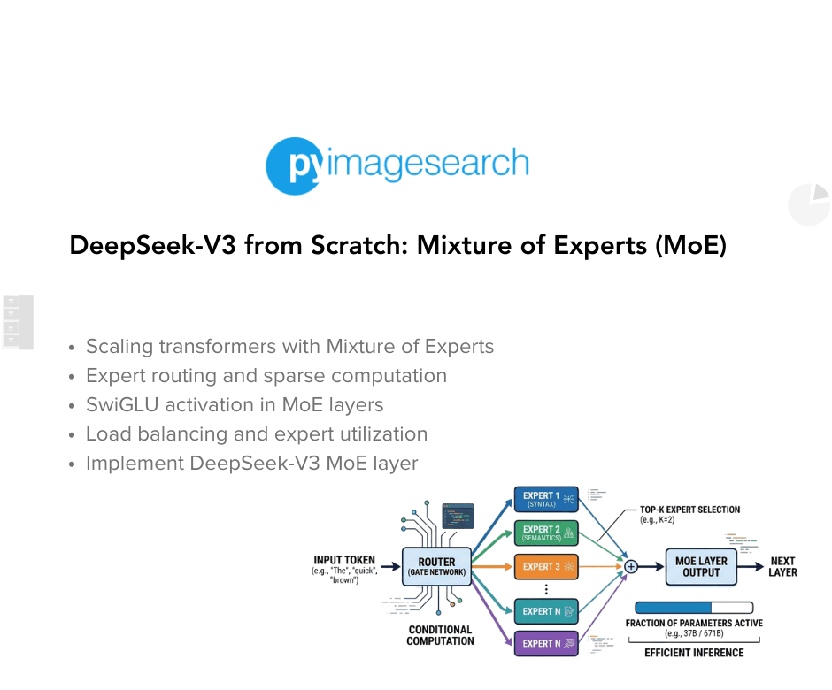
Mixture of Experts (Figure 1) offers a more efficient scaling paradigm: instead of a single large FFN, we create multiple smaller expert FFNs and route each token to a subset of these experts. This gives us the capacity of a much larger model while maintaining computational efficiency.

---

Mixture of Experts (MoE): Mathematical Foundation and Routing Mechanism

Consider expert networks, each with the same architecture as a standard FFN:

for . Instead of using all experts for every token, we select the top-k experts. The selection is determined by a learned routing function:

where is the router weight matrix and is a learnable bias vector. This gives us a probability distribution over experts for each token.

Top-k Routing: We select the top-k experts based on router probabilities:

The final output combines the selected experts, weighted by their normalized routing probabilities:

The renormalization ensures the selected experts’ weights sum to 1.

Capacity and Computation: With experts and (our configuration), each token activates 2 out of 4 experts. If each expert has the same size as a standard FFN, we have the parameters but only the computation per token. This is the MoE efficiency advantage: parameter count scales with , but computation scales with .

---

SwiGLU Activation in DeepSeek-V3: Improving MoE Non-Linearity

DeepSeek uses SwiGLU (Swish-Gated Linear Unit) instead of the traditional GELU (Gaussian Error Linear Units) activation. SwiGLU is a gated activation function that has shown superior performance in language models:

where:

• : projects input to hidden dimension
• : is another projection to hidden dimension
• : is the Swish activation (smooth version of ReLU)
• : denotes element-wise multiplication
• The result is then projected back:

The gating mechanism allows the network to control information flow more precisely than simple activation functions. The activation provides smooth gradients everywhere, improving training dynamics compared to ReLU’s hard threshold.

---

Shared Expert in DeepSeek-V3: Universal Processing in MoE Layers

DeepSeek introduces a shared expert that processes all tokens in addition to the routed experts. This design addresses a key limitation of pure MoE: some computations are beneficial for all tokens regardless of their content.

The shared expert has a larger hidden dimension (768 in our configuration vs 512 for individual experts) and processes every token. This ensures that:

• Common patterns are efficiently handled by dedicated capacity
• Specialized experts can focus on token-specific features
• Training is more stable with guaranteed gradient flow

The shared expert serves as a “base” computation that’s always present, while routed experts add specialized processing on top of it.

---

Auxiliary-Loss-Free Load Balancing in DeepSeek-V3 MoE

A critical challenge in MoE is load balancing. If the router learns to always send tokens to the same one or two experts, we lose the benefits of having multiple experts — the unused experts contribute nothing, and the overused ones become bottlenecks.

Traditional MoE models use an auxiliary loss that penalizes uneven expert usage:

where is the number of tokens routed to expert , is batch size, and is a coefficient. However, auxiliary losses add complexity and require careful tuning.

DeepSeek’s Innovation: Auxiliary-loss-free load balancing through dynamic bias updates. Instead of penalizing imbalance during training, we adjust the router biases to encourage balanced usage:

During training, we monitor how many tokens are routed to each expert. This gives us an expert_usage vector, where each entry counts the number of tokens assigned to a particular expert. We then compute the average usage across all experts.

To maintain a balanced load, we adjust the router biases: if an expert is used more than the average, its bias is decreased to make it less likely to be chosen in the future; if it is used less than the average, its bias is increased to make it more likely to be selected. This dynamic bias update encourages fair distribution of tokens across experts without requiring an explicit auxiliary loss.

Let denote the usage (number of tokens) of expert , and let

be the average usage across all experts. The router bias for expert , denoted , is updated as:

,

where is the learning rate controlling the magnitude of the bias adjustment.

This approach:

• Eliminates the need for auxiliary loss hyperparameter tuning
• Provides smoother load balancing over time
• Doesn’t interfere with the primary task loss
• Automatically adapts to data distribution changes

The bias updates are performed with a small learning rate (0.001 in our implementation) to ensure gradual adjustment without disrupting training.

---

Sequence-Wise Load Balancing for Mixture of Experts Models

For even better load balancing, DeepSeek can use a complementary sequence-wise auxiliary loss. This encourages different sequences in a batch to use different experts:

,

where is the expert usage vector for sequence (i.e., which experts were used), and measures similarity. By minimizing this loss, we encourage sequences to be complementary — if sequence A uses experts 1 and 2 heavily, sequence B should use experts 3 and 4.

---

Expert Specialization in MoE: Emergent Behavior in DeepSeek-V3

A fascinating property of MoE is expert specialization. Even though we don’t explicitly tell experts what to specialize in, they often learn to handle different types of patterns. In language models, researchers have observed:

• Syntactic experts: Handle grammatical structures, verb conjugations
• Semantic experts: Process meaning, synonyms, and conceptual relationships
• Domain experts: Specialize in specific topics (e.g., scientific text, dialogue)
• Numerical experts: Handle arithmetic, dates, quantities

This specialization emerges naturally as the routing function learns which experts are most effective for different inputs. Gradient flow during training reinforces this — when an expert performs well on certain patterns, the router learns to send similar patterns to that expert.

Mathematically, we can think of each expert as learning a local model that’s particularly good in some region of the input space. The router function implicitly partitions the input space, assigning different regions to different experts. This is similar to a mixture of experts in classical machine learning, but learned end-to-end through backpropagation.

---

Implementation: Building the DeepSeek-V3 MoE Layer from Scratch

Let’s implement the complete MoE layer with expert networks, routing, and load balancing:

class SwiGLU(nn.Module):
    """SwiGLU activation function used in DeepSeek experts"""
   
    def __init__(self, input_dim: int, hidden_dim: int, output_dim: int, bias: bool = True):
        super().__init__()
        self.gate_proj = nn.Linear(input_dim, hidden_dim, bias=bias)
        self.up_proj = nn.Linear(input_dim, hidden_dim, bias=bias)
        self.down_proj = nn.Linear(hidden_dim, output_dim, bias=bias)
       
    def forward(self, x: torch.Tensor):
        gate = F.silu(self.gate_proj(x))  # SiLU activation
        up = self.up_proj(x)
        return self.down_proj(gate * up)

Lines 1-13: SwiGLU Activation: The SwiGLU class implements a gated activation mechanism. We have 3 linear projections:

• gate_proj: for the gating signal
• up_proj: for the value branch
• down_proj: for the output projection

The forward pass applies SiLU (Sigmoid Linear Unit) to the gate projection, multiplies it element-wise with the up-projection, and projects back down. This creates a more expressive activation than simple GELU, with the gating mechanism allowing fine-grained control over information flow.

class MoEExpert(nn.Module):
    """Expert network for Mixture of Experts using SwiGLU"""

    def __init__(self, config: DeepSeekConfig):
        super().__init__()
        self.expert_mlp = SwiGLU(
            config.n_embd,
            config.expert_intermediate_size,
            config.n_embd,
            config.bias
        )

    def forward(self, x: torch.Tensor):
        return self.expert_mlp(x)

Lines 14-27: Expert with SwiGLU: Each MoEExpert is now a SwiGLU network instead of a simple FFN. The intermediate size (expert_intermediate_size) controls capacity — we use 512 in our configuration, which is smaller than the shared expert’s 768. This asymmetry reflects the fact that routed experts handle specialized patterns, while the shared expert handles common operations.

class MixtureOfExperts(nn.Module):
    """
    DeepSeek MoE layer with shared expert and auxiliary-loss-free load balancing
   
    Key features:
    - Shared expert that processes all tokens
    - Auxiliary-loss-free load balancing via bias updates
    - Top-k routing to selected experts
    """

    def __init__(self, config: DeepSeekConfig):
        super().__init__()
        self.config = config
        self.n_experts = config.n_experts
        self.top_k = config.n_experts_per_token
        self.n_embd = config.n_embd

        # Router: learns which experts to use for each token
        self.router = nn.Linear(config.n_embd, config.n_experts, bias=False)

        # Expert networks
        self.experts = nn.ModuleList([
            MoEExpert(config) for _ in range(config.n_experts)
        ])

        # Shared expert (processes all tokens)
        if config.use_shared_expert:
            self.shared_expert = SwiGLU(
                config.n_embd,
                config.shared_expert_intermediate_size,
                config.n_embd,
                config.bias
            )
        else:
            self.shared_expert = None

        # Auxiliary-loss-free load balancing
        self.register_buffer('expert_bias', torch.zeros(config.n_experts))
        self.bias_update_rate = 0.001

        self.dropout = nn.Dropout(config.dropout)

Lines 28-68: MoE Layer Structure: The MixtureOfExperts class orchestrates routing and expert execution. The 3 key additions:

• shared_expert: full-capacity expert that processes all tokens
• expert_bias: buffer for auxiliary-loss-free balancing
• bias_update_rate: controls how quickly biases adapt

The dropout provides regularization across the entire MoE output.

    def forward(self, x: torch.Tensor):
        batch_size, seq_len, hidden_dim = x.shape
        x_flat = x.view(-1, hidden_dim)

        # Routing phase with bias for load balancing
        router_logits = self.router(x_flat) + self.expert_bias

        # Top-k routing
        top_k_logits, top_k_indices = torch.topk(router_logits, self.top_k, dim=-1)
        routing_weights = torch.zeros_like(router_logits)
        routing_weights.scatter_(-1, top_k_indices, F.softmax(top_k_logits, dim=-1))

        # Expert computation
        output = torch.zeros_like(x_flat)
        expert_usage = torch.zeros(self.n_experts, device=x.device)

Lines 70-84: Routing with Learnable Bias. The forward pass begins by flattening the input for efficient processing. We compute router logits and add the expert bias — this is the key to auxiliary-loss-free balancing. Overused experts have negative bias (making them less likely to be selected), while underused experts have positive bias (encouraging them to be selected). We then perform top-k selection and softmax normalization across the selected experts.

        # Process through selected experts
        for expert_idx in range(self.n_experts):
            expert_mask = (top_k_indices == expert_idx).any(dim=-1)
            expert_usage[expert_idx] = expert_mask.sum().float()

            if expert_mask.any():
                expert_input = x_flat[expert_mask]
                expert_output = self.experts[expert_idx](expert_input)

                # Weight by routing probability
                weights = routing_weights[expert_mask, expert_idx].unsqueeze(-1)
                output[expert_mask] += expert_output * weights

        # Add shared expert output (processes all tokens)
        if self.shared_expert is not None:
            shared_output = self.shared_expert(x_flat)
            output += shared_output

        # Auxiliary-loss-free load balancing (update biases during training)
        if self.training:
            with torch.no_grad():
                avg_usage = expert_usage.mean()
                for i in range(self.n_experts):
                    if expert_usage[i] > avg_usage:
                        self.expert_bias[i] -= self.bias_update_rate
                    else:
                        self.expert_bias[i] += self.bias_update_rate

        output = self.dropout(output)
        return output.view(batch_size, seq_len, hidden_dim), router_logits.view(batch_size, seq_len, -1)

Lines 86-97: Expert Processing. We iterate over all experts, identifying which tokens route to each one via the expert_mask. For each expert with assigned tokens, we extract those tokens, process them through the expert network, weight them by routing probability, and accumulate them into the output. This selective execution is what makes MoE efficient — we don’t compute all experts for all tokens.

Lines 100-102: Shared Expert. The shared expert processes all tokens unconditionally and adds its output to the routed experts’ output. This ensures every token receives some baseline processing, improving training stability and providing capacity for universal patterns. The shared expert’s larger hidden dimension (768 vs 512) reflects its broader responsibility.

Lines 105-112: Auxiliary-Loss-Free Balancing. During training, we update expert biases based on usage. We compute average usage across experts, then adjust biases: overused experts receive negative adjustments (discouraging future selection), while underused experts receive positive adjustments (encouraging future selection). Using the torch.no_grad() context ensures these bias updates don’t interfere with gradient computation. The small update rate (0.001) provides smooth, stable balancing over time.

Lines 114-115: Output and Return. We apply dropout to the combined output (routed + shared experts) and reshape back to the original dimensions. We return both the output and router logits — the latter can be used for optional auxiliary loss computation.

    def _complementary_sequence_aux_loss(self, router_logits, seq_mask=None):
      """
      router_logits: [batch_size, seq_len, num_experts]
          Raw logits from the router before softmax.
      seq_mask: optional mask for padding tokens.
      """

      # Convert to probabilities
      probs = F.softmax(router_logits, dim=-1)  # [B, T, E]

      # Aggregate per-sequence expert usage
      if seq_mask is not None:
          probs = probs * seq_mask.unsqueeze(-1)  # mask padding
      seq_usage = probs.sum(dim=1)  # [B, E]

      # Normalize per sequence
      seq_usage = seq_usage / seq_usage.sum(dim=-1, keepdim=True)

      # Compute pairwise similarity between sequences
      sim_matrix = torch.matmul(seq_usage, seq_usage.transpose(0, 1))  # [B, B]

      # Encourage complementarity: minimize similarity off-diagonal
      batch_size = seq_usage.size(0)
      off_diag = sim_matrix - torch.eye(batch_size, device=sim_matrix.device)
      loss = off_diag.mean()

      return loss

Lines 117-143: Complementary Sequence-Wise Loss. This method implements an alternative load-balancing approach. It converts router logits to probabilities, aggregates expert usage for each sequence, and computes pairwise similarity between sequences’ expert usage patterns. By minimizing off-diagonal similarity, we encourage different sequences to use different experts, promoting diversity in expert utilization. This can be added to the training loss with a small weight (e.g., 0.01).

---

MoE Design Decisions in DeepSeek-V3: SwiGLU, Shared Experts, and Routing

Several implementation choices merit discussion:

SwiGLU vs GELU: We use SwiGLU instead of traditional GELU because empirical research shows it consistently outperforms GELU in language models. The gating mechanism provides more expressive power, and SiLU’s smoothness improves gradient flow. The computational cost is slightly higher (three projections instead of two), but the quality improvement justifies it.

Shared Expert Design: The shared expert is a DeepSeek innovation that addresses a key limitation of pure MoE: some computations benefit all tokens. By providing dedicated capacity for universal processing, we free routed experts to specialize more aggressively. The larger hidden dimension (768 vs 512) for the shared expert reflects empirical findings that shared capacity requires more parameters than individual experts.

Auxiliary-Loss-Free Balancing: Traditional MoE uses auxiliary losses, such as:

where is the fraction of tokens routed to expert and is the average routing probability. This requires tuning (typically 0.01-0.1). Our bias-based approach eliminates the need for this hyperparameter, simplifying training. The tradeoff is that bias updates are less direct than gradient-based learning, but in practice, the smoother adaptation works well.

Complementary Sequence-Wise Loss: This alternative balancing approach is useful when batch diversity is high. By encouraging different sequences to use different experts, we naturally achieve balance. However, if the batch contains very similar sequences (e.g., all from the same domain), this loss may not be effective. It’s best used in combination with bias-based balancing or as an optional auxiliary objective.

Expert Capacity: Production MoE systems often implement expert capacity constraints — if too many tokens route to one expert, excess tokens are dropped or routed to a second choice. We don’t implement this in our educational model, but the formula would be:

where factor is typically 1.25-1.5. Tokens beyond this capacity are handled via overflow strategies.

---

MoE Computational and Memory Analysis in DeepSeek-V3

Let’s analyze the computational cost. For a standard FFN with hidden dimension :

For our MoE with routed experts (each with ), selected, and shared expert ():

The SwiGLU computation involves three projections:

For our configuration:

• Routing: (negligible)
• Routed experts:
• Shared expert:
• Total: 2.75M FLOPs per token

Compare to a standard FFN with : FLOPs. Our MoE uses 2.6× more computation but has much higher capacity (4 experts × 512 + 1 shared × 768 = 2,816 vs 1,024). We get 2.7× capacity for 2.6× computation — roughly linear scaling, which is the goal.

Memory usage during the forward pass stores activations for active experts only. During backpropagation, we need gradients for all experts (since routing is differentiable), yet the memory remains manageable. The bias vector is tiny (4 floats for 4 experts).

---

MoE Expert Specialization in Practice: Real-World Behavior

While we can’t demonstrate this in our small toy model, in larger-scale MoE models, expert specialization is observable through analysis of routing patterns. Researchers have visualized which experts activate for different types of inputs, revealing clear specialization. For example:

• Multilingual models: Different experts handle different languages
• Code models: Some experts handle syntax, others semantics, others API patterns
• Reasoning models: Numerical experts for math, logical experts for inference, retrieval experts for factual recall

This specialization isn’t programmed — it emerges from optimization. The routing function learns to partition the input space, and experts learn to excel in their assigned partitions. It’s a beautiful example of how end-to-end learning can discover structured solutions.

---

Training Dynamics of MoE: Load Balancing and Expert Utilization

In practice, MoE training exhibits interesting dynamics:

Early Training: Routing is initially random or near-uniform. All experts receive a similar load. The shared expert learns basic patterns that benefit all tokens.

Mid Training: Routing starts specializing. Some experts become preferred for certain patterns. Load imbalance can emerge without careful management. Bias-based balancing begins correcting the imbalance.

Late Training: Experts are clearly specialized. Routing is confident (high softmax probabilities for selected experts). Load is balanced through continuous bias adjustment. The shared expert handles universal operations while routed experts focus on specialized patterns.

Monitoring expert usage during training is valuable. We can log:

• Per-expert selection frequency
• Routing entropy (higher means more uniform)
• Expert bias magnitudes (large values indicate strong correction needed)

---

Mixture of Experts vs Related Techniques: Switch Transformers and Sparse Models

MoE shares ideas with several other architectural patterns:

Switch Transformers: Use top-1 routing (only one expert per token) for maximum efficiency. Simpler but less expressive than top-k.

Expert Choice: Instead of tokens choosing experts, experts choose tokens. Helps with load balancing but changes the computational pattern.

Sparse Attention: Like MoE, selectively activates parts of the network. Can be combined with MoE for extreme efficiency.

Dynamic Networks: Adapt network structure based on input. MoE is a specific form of dynamic computation.

With our MoE implementation complete, we’ve added efficient scaling to our model — the capacity grows superlinearly with computation cost. Combined with MLA’s memory efficiency and the upcoming MTP’s improved training signal, we’re building a model that’s efficient in training, efficient in inference, and capable of strong performance. Next, we’ll tackle Multi-Token Prediction, which improves the training signal itself by having the model look further ahead.

---

---

Summary

In the third installment of our DeepSeek-V3 from Scratch series, we turn our attention to the Mixture of Experts (MoE) framework, a powerful approach to scaling neural networks efficiently. We begin by unpacking the scaling challenge in modern architectures and how MoE addresses it through selective expert activation. From its mathematical foundation to the introduction of SwiGLU activation, we explore how enhanced non-linearity and universal shared experts contribute to more flexible and expressive models.

We then examine the mechanics of load balancing, highlighting innovations (e.g., auxiliary-loss-free balancing and complementary sequence-wise strategies). These techniques ensure that experts are used effectively without introducing unnecessary complexity. We also explore how expert specialization emerges naturally during training, leading to diverse behaviors across experts that improve overall performance. This emergent specialization is not just theoretical — it becomes visible in practice, shaping how the model processes different types of input.

Finally, we walk through the implementation of MoE, discussing design decisions, computational trade-offs, and memory analysis. We connect these insights to related techniques, showing how MoE integrates into the broader landscape of efficient deep learning. By the end, we not only understand the theory but also gain practical knowledge of how to implement and optimize MoE within DeepSeek-V3. This part of the series equips us with the tools to harness expert specialization while keeping training dynamics balanced and efficient.

---

Citation Information

Mangla, P. “DeepSeek-V3 from Scratch: Mixture of Experts (MoE),” PyImageSearch, S. Huot, A. Sharma, and P. Thakur, eds., 2026, https://pyimg.co/a1w0g

@incollection{Mangla_2026_deepseek-v3-from-scratch-moe,
  author = {Puneet Mangla},
  title = {{DeepSeek-V3 from Scratch: Mixture of Experts (MoE)}},
  booktitle = {PyImageSearch},
  editor = {Susan Huot and Aditya Sharma and Piyush Thakur},
  year = {2026},
  url = {https://pyimg.co/a1w0g},
}

---

To download the source code to this post (and be notified when future tutorials are published here on PyImageSearch), simply enter your email address in the form below!

The post DeepSeek-V3 from Scratch: Mixture of Experts (MoE) appeared first on PyImageSearch.