Building a Temporal Knowledge Graph with Python and NetworkX

Authors:
Shon Mohsin, D. Eng AI
Jeremiah Lowhorn, D. Eng AI
Seth Thor
Matthew Morais, D. Eng AI

What if you could ask your data: “What did we know about this research topic in June 2024?” — and get a precise, structured answer?

Scientific Research generates a web of interconnected entities — subjects, methods, outcomes, organizations, publications — that evolves over time. A spreadsheet can track individual facts. A relational database can join tables. But neither preserves the shape of knowledge: the web of typed relationships between entities that grows and changes with every new publication.

Knowledge graphs do.

In this article, we’ll build a temporal knowledge graph in Python using NetworkX. It ingests scientific publications, extracts entities, wires them into a typed graph, and supports “time-travel” queries — answering questions about what was known at any point in the past. The implementation uses a scientific research domain, but the patterns transfer directly to supply chain tracking, legal document analysis, financial intelligence, and any field where relationships between entities matter more than the entities themselves.

What Is a Knowledge Graph?

A knowledge graph is a data structure where nodes represent entities and edges represent typed relationships between them. Both nodes and edges carry attributes.

This sounds like a regular graph, but the key distinction is typing. In a simple graph, nodes are nodes and edges are edges. In a knowledge graph:

• Nodes have types: a Publication node is fundamentally different from a Drug node or a Target node
• Edges have types: a DESCRIBES_DRUG edge is different from a TARGETS edge or a TREATS edge
• Both carry attributes: a publication has a timestamp, a drug has a development stage, a relationship has a date it was established

This is what separates a knowledge graph from a relational database. In a relational model, you’d represent these as separate tables with foreign keys. In a KG, the relationships are first-class citizens — you can traverse, query, and reason over them directly.

Real-world examples include Google’s Knowledge Graph (powering search cards), Wikidata (structured Wikipedia), and biomedical KGs like Hetionet. Increasingly, knowledge graphs serve as structured retrieval layers for LLM-based systems, providing context that vector similarity search alone cannot capture.

If we add temporal awareness — timestamps on edges and the ability to filter by time — the knowledge graph becomes a time machine for your domain.

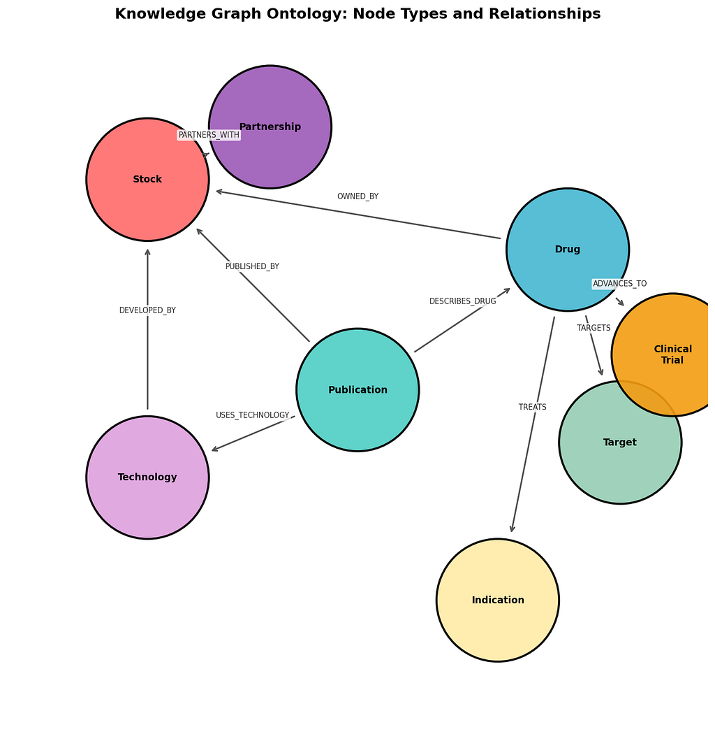
Step 1: Design the Ontology

Every knowledge graph starts with an ontology: the schema that defines what types of entities and relationships your graph can contain. Think of it as the blueprint before construction.

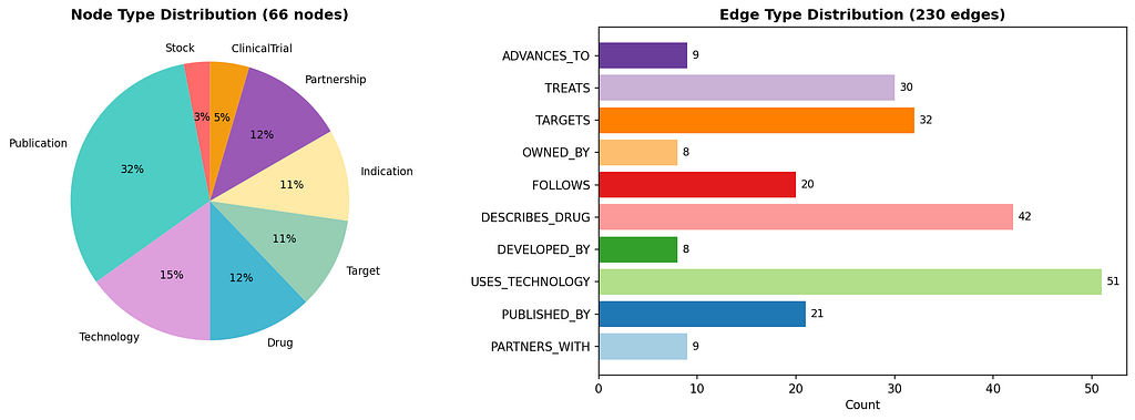
For our scientific publications graph, we define 8 node types and 10 relationship types:

from enum import Enum

class NodeType(Enum):
    STOCK = "Stock"               # Organizations / companies
    PUBLICATION = "Publication"    # Source documents
    DRUG = "Drug"                 # Research subjects
    TARGET = "Target"             # Biological targets
    INDICATION = "Indication"     # Disease areas
    TECHNOLOGY = "Technology"     # Methods and platforms
    CLINICAL_TRIAL = "ClinicalTrial"
    PARTNERSHIP = "Partnership"

class EdgeType(Enum):
    PUBLISHED_BY = "PUBLISHED_BY"       # Publication -> Organization
    DESCRIBES_DRUG = "DESCRIBES_DRUG"   # Publication -> Subject
    TARGETS = "TARGETS"                 # Subject -> Target
    TREATS = "TREATS"                   # Subject -> Disease
    USES_TECHNOLOGY = "USES_TECHNOLOGY" # Publication -> Technology
    ADVANCES_TO = "ADVANCES_TO"        # Subject -> Study
    PARTNERS_WITH = "PARTNERS_WITH"    # Organization -> Partnership
    FOLLOWS_TEMPORALLY = "FOLLOWS"     # Publication -> Publication
    OWNED_BY = "OWNED_BY"             # Subject -> Organization
    DEVELOPED_BY = "DEVELOPED_BY"     # Technology -> Organization

Each node type is backed by a Python dataclass that defines its attributes and provides serialization:

from dataclasses import dataclass, field
from typing import Optional, List

@dataclass
class DrugNode:
    drug_id: str
    name: str
    code: Optional[str] = None
    mechanism: Optional[str] = None
    stage: DrugStage = DrugStage.DISCOVERY
    therapeutic_area: Optional[TherapeuticArea] = None

    @property
    def node_id(self) -> str:
        return self.drug_id

    @property
    def node_type(self) -> NodeType:
        return NodeType.DRUG

    def to_dict(self) -> dict:
        return {
            "node_type": self.node_type.value,
            "drug_id": self.drug_id,
            "name": self.name,
            "code": self.code,
            "mechanism": self.mechanism,
            "stage": self.stage.value,
            "therapeutic_area": self.therapeutic_area.value if self.therapeutic_area else None,
        }

The key design decisions here:

1. Enums for controlled vocabularies — node types, edge types, development stages, and therapeutic areas are all enums. This prevents typos from creating ghost categories and makes the ontology self-documenting.
2. Dataclasses for structure — each entity type has explicit fields with types and defaults, making the schema clear to any contributor.
3. to_dict() for serialization – every node can flatten itself into a dictionary for graph storage or JSON export.

Step 2: Parse Unstructured Data into Entities

Knowledge graphs don’t build themselves. The hardest part is going from unstructured documents to structured entities. Our implementation takes a pragmatic approach: a combination of filename conventions and regex-based entity extraction.

Each publication file follows a naming convention that encodes metadata:

YYYYMMDD_ORG_Topic_Source.md

The parser extracts timestamp, organization ticker, and source type from the filename alone:

def parse_filename(filename: str) -> dict:
    base = filename.replace('.md', '').replace('.pdf', '')
    parts = base.split('_')

    date_str = parts[0]
    year, month, day = int(date_str[:4]), int(date_str[4:6]), int(date_str[6:8])
    timestamp = datetime(year, month, max(1, day))

    ticker = parts[1]
    source = parts[-1]
    pub_type = _infer_publication_type(source, filename)
    return {'timestamp': timestamp, 'ticker': ticker, 'source': source, 'pub_type': pub_type}

For entity extraction from document content, the system uses regex patterns matched against known entities:

def _extract_drugs(content: str) -> list:
    drugs = []
    drug_patterns = [
        (r'zovegalisib|RLY-2608', 'Zovegalisib', 'RLY-2608',
         'Allosteric inhibitor', DrugStage.PHASE3, TherapeuticArea.ONCOLOGY),
        (r'REC-994|tempol', 'REC-994', 'REC-994',
         'Redox-cycling nitroxide', DrugStage.PHASE2, TherapeuticArea.NEUROLOGY),
        # ... more patterns
    ]
    for pattern, name, code, mechanism, stage, area in drug_patterns:
        if re.search(pattern, content, re.IGNORECASE):
            drugs.append({'name': name, 'code': code, 'mechanism': mechanism,
                          'stage': stage, 'therapeutic_area': area})
    return drugs

The same pattern-matching approach applies to targets (gene symbols), indications (disease names), technologies (platform names), clinical trials, and partnerships.

Trade-off note: Regex-based extraction is deterministic and precise for a bounded domain with known entities. For open-domain extraction at scale, you’d swap in NLP/NER models (spaCy, biomedical BERT, etc.). The graph builder doesn’t care how entities are extracted — it just needs structured dictionaries.

Step 3: Build the Graph with NetworkX

With the ontology defined and the parser producing structured data, we can build the graph. We use NetworkX’s MultiDiGraph – a directed graph that allows multiple edges between the same pair of nodes (essential when a publication both DESCRIBES_DRUG and USES_TECHNOLOGY connected to the same entity).

The core class maintains tracking dictionaries for deduplication:

import networkx as nx

class BiotechKnowledgeGraph:
    def __init__(self):
        self.graph = nx.MultiDiGraph()
        self._drugs = {}
        self._targets = {}
        self._publications = {}
        # ... tracking dicts for each node type

The central method processes a parsed publication and creates all nodes and edges:

def add_publication_with_entities(self, parsed_data: dict):
    timestamp = parsed_data.get('timestamp')
    ticker = parsed_data.get('ticker')

    # Create publication node
    pub_id = f"pub_{parsed_data['filename'].replace('.md', '')}"
    pub = PublicationNode(pub_id=pub_id, timestamp=timestamp, ...)
    self._add_publication(pub)

    # Link publication to organization
    self._add_edge(pub_id, ticker, EdgeType.PUBLISHED_BY, timestamp)

    # Process each entity type and create relationships
    for drug_data in parsed_data.get('drugs', []):
        drug_id = self._add_drug(drug_data)
        self._add_edge(pub_id, drug_id, EdgeType.DESCRIBES_DRUG, timestamp)
        self._add_edge(drug_id, ticker, EdgeType.OWNED_BY, timestamp)

        for target_data in parsed_data.get('targets', []):
            target_id = self._add_target(target_data)
            self._add_edge(drug_id, target_id, EdgeType.TARGETS, timestamp)

        for indication_data in parsed_data.get('indications', []):
            indication_id = self._add_indication(indication_data)
            self._add_edge(drug_id, indication_id, EdgeType.TREATS, timestamp)

    for tech_data in parsed_data.get('technologies', []):
        tech_id = self._add_technology(tech_data)
        self._add_edge(pub_id, tech_id, EdgeType.USES_TECHNOLOGY, timestamp)

Notice that every edge carries a timestamp. This is the foundation for temporal queries.

After all publications are ingested, we create temporal chains — FOLLOWS_TEMPORALLY edges that link publications about the same research subject in chronological order:

def add_temporal_edges(self):
    drug_pubs = defaultdict(list)
    for pub_id, pub in self._publications.items():
        for _, target, data in self.graph.out_edges(pub_id, data=True):
            if data.get('edge_type') == EdgeType.DESCRIBES_DRUG.value:
                drug_pubs[target].append((pub.timestamp, pub_id))

    for drug_id, pubs in drug_pubs.items():
        sorted_pubs = sorted(pubs, key=lambda x: x[0])
        for i in range(len(sorted_pubs) - 1):
            self._add_edge(
                sorted_pubs[i][1], sorted_pubs[i + 1][1],
                EdgeType.FOLLOWS_TEMPORALLY, sorted_pubs[i + 1][0],
                context=f"drug:{drug_id}"
            )

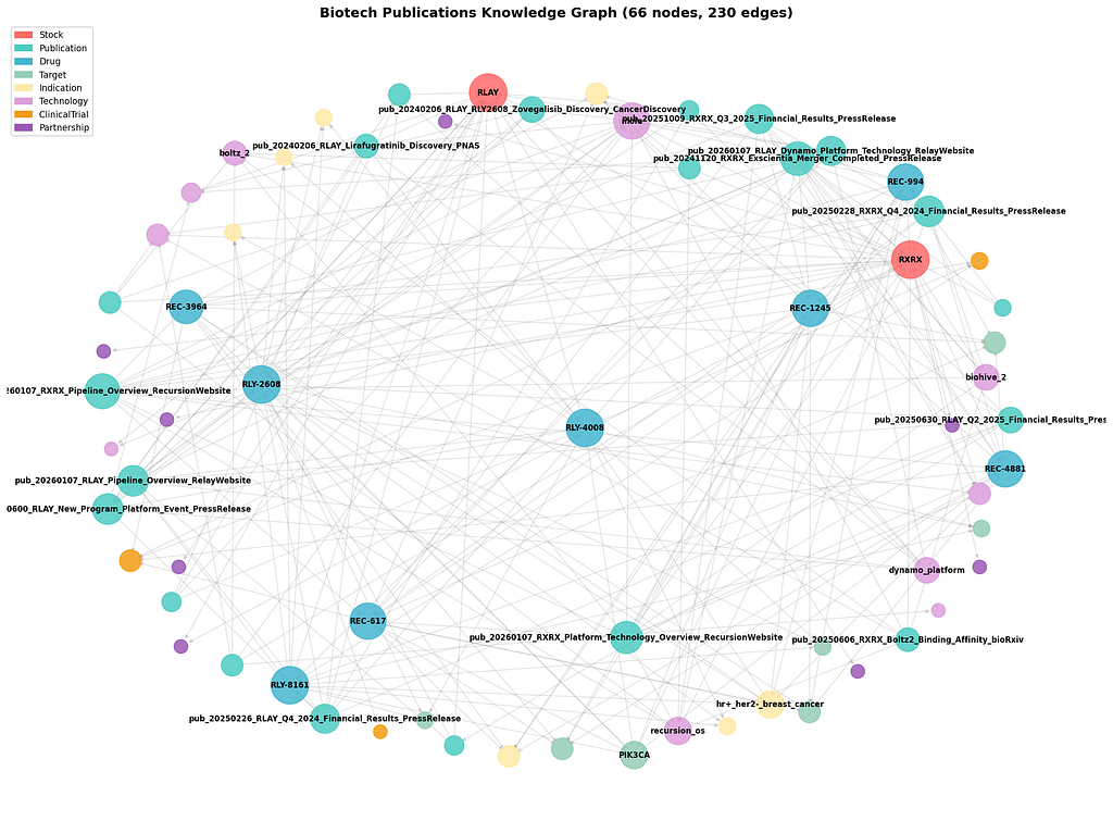
A single publication typically generates 10+ nodes and edges. From ~20 documents, our graph reached 66 nodes and 230 edges.

Step 4: Time-Travel Queries — The Killer Feature

What makes this a temporal knowledge graph is the ability to ask: “What was known at date X?”

The TemporalQueryEngine class wraps the graph with time-aware query methods:

Historical Snapshot

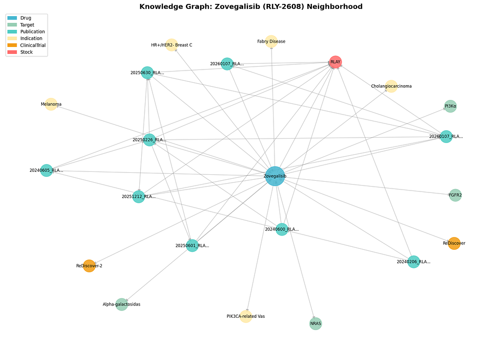
The most powerful query reconstructs the known state of any entity at a specific point in time:

def get_drug_state_at_date(self, drug_id: str, as_of_date: datetime) -> dict:
    drug_data = dict(self.graph.nodes[drug_id])
    timeline = self.get_drug_timeline(drug_id)

    relevant_pubs = [p for p in timeline if p['timestamp'] <= as_of_date]

    known_targets, known_indications, known_trials = set(), set(), set()

    for source, target, data in self.graph.out_edges(drug_id, data=True):
        edge_ts = datetime.fromisoformat(data.get('timestamp', ''))
        if edge_ts > as_of_date:
            continue

        edge_type = data.get('edge_type')
        if edge_type == EdgeType.TARGETS.value:
            known_targets.add(target)
        elif edge_type == EdgeType.TREATS.value:
            known_indications.add(target)
        elif edge_type == EdgeType.ADVANCES_TO.value:
            known_trials.add(target)

    return {
        'drug_id': drug_id,
        'publication_count': len(relevant_pubs),
        'known_targets': list(known_targets),
        'known_indications': list(known_indications),
        'known_trials': list(known_trials),
    }

This simulates the information landscape at any historical date. Useful for backtesting research decisions, regulatory analysis, or understanding how knowledge accumulates over time.

Time-Constrained Path Finding

Perhaps the most interesting query: find paths between two entities using only edges that existed before a cutoff date:

def find_paths_before_date(self, source: str, target: str,
                            cutoff_date: datetime, max_depth: int = 4) -> list:
    # Build subgraph with only pre-cutoff edges
    valid_edges = []
    for u, v, key, data in self.graph.edges(keys=True, data=True):
        edge_ts_str = data.get('timestamp')
        if not edge_ts_str or datetime.fromisoformat(edge_ts_str) <= cutoff_date:
            valid_edges.append((u, v, key))

    subgraph = nx.MultiDiGraph()
    subgraph.add_nodes_from(self.graph.nodes(data=True))
    for u, v, key in valid_edges:
        subgraph.add_edge(u, v, key=key, **self.graph.edges[u, v, key])

    return list(nx.all_simple_paths(subgraph, source, target, cutoff=max_depth))

This answers questions like: “Could we have connected research subject A to disease B based on what was published before March 2024?” — a powerful tool for analyzing information flow and research gaps.

Other Temporal Queries

The engine also supports:

• Entity timelines: chronological list of all publications about a subject
• Organization comparison: compare pipeline sizes, tech stacks, and publication activity at any date
• Publication counts by month: track research activity trends over time
• Development stage progression: track how a subject’s status evolved through publications

Step 5: Serialize and Visualize

The graph exports to four formats, each serving a different use case:

def save(self, output_dir: str, name: str = "biotech_kg"):
    # Pickle -- full Python object, best for reloading
    with open(f"{name}.pickle", 'wb') as f:
        pickle.dump(self.graph, f)

    # GraphML -- interoperable with Gephi, Cytoscape, yEd
    nx.write_graphml(G_export, f"{name}.graphml")

    # JSON -- D3.js-ready for web visualization
    self._save_as_json(f"{name}.json")

    # Stats JSON -- summary metrics
    json.dump(self.get_statistics(), f)

For visualization, the GraphML export works directly with Gephi (network analysis) or Cytoscape (biological networks). The JSON export is structured for D3.js force-directed layouts. For quick Python visualization, pyvis can render interactive HTML graphs from NetworkX directly.

What We Built

From approximately 20 scientific publication documents, the system extracted:

+--------------------+----------+
| Metric             | Count    |
+--------------------+----------+
| Total nodes        | 66       |
| Total edges        | 230      |
| Node types         | 8        |
| Edge types         | 10       |
| Publications       | 21       |
| Research subjects  | 8        |
| Technologies       | 10       |
| Biological targets | 7        |
| Disease areas      | 7        |
| Partnerships       | 8        |
| Clinical studies   | 3        |
| Temporal range     | 3+ years |
+--------------------+----------+

The graph answers questions that no single document, spreadsheet, or database table can:

• What was the state of knowledge about subject X at date Y?
• How did an organization’s research pipeline evolve over time?
• What technologies were associated with which publications?
• What paths connect two entities through the graph?

Where to Go From Here

This implementation is a foundation. Here’s how to extend it:

1. NLP-based entity extraction — Replace regex patterns with spaCy or domain-specific NER models for open-domain extraction at scale
2. Graph database backend — Swap NetworkX for Neo4j or Amazon Neptune when the graph outgrows memory
3. Graph algorithms — Run centrality analysis (which entity is most connected?), community detection (which entities cluster together?), or link prediction (what connections are likely missing?)

1. RAG integration — Use the knowledge graph as a structured retrieval layer for LLM-based question answering, combining graph traversal with semantic search
2. Collaboration networks — Add author and institution nodes to map who works with whom across publications

Conclusion

Knowledge graphs aren’t just for Google. They’re a practical data structure for anyone dealing with complex, evolving relationships — from research intelligence to supply chains to legal document analysis.

The combination of typed nodes, typed edges, temporal awareness, and graph traversal gives you a fundamentally different tool than relational databases or flat files. You don’t just store facts — you store the structure of knowledge, and you can query that structure across time.

The full implementation is available in the project repository. The entire system runs on Python standard library plus NetworkX — no database server, no cloud service, no heavyweight dependencies.

Think about your own domain. What entities do you track? What relationships between them are you currently losing to flat data structures? That’s where your knowledge graph begins.

Built with Python 3, NetworkX, and dataclasses. No external database required.

For questions, please email us at shon@numenai.capital

---

Building a Temporal Knowledge Graph with Python and NetworkX was originally published in Towards AI on Medium, where people are continuing the conversation by highlighting and responding to this story.