
Behind the Scenes of Bias Variance Trade-Off and L1 , L2 Regularization
🎯 The Core of Machine Learning: Bias-Variance Trade-off
Before we dive into how to fix our models with regularization, we have to understand the two “ghosts” that haunt every machine learning algorithm: Bias and Variance.
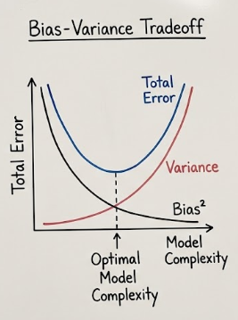
Every time we train a model, we are trying to minimize the Total Error. As your notes correctly show, this error is composed of three parts:
- Bias² (Reducible)
- Variance (Reducible)
- Irreducible Error (Noise that we can’t do anything about)
1. What is Bias? (The “Underfitter”)
Bias is the error introduced by approximating a real-life problem (which is usually complicated) with a much simpler model.

- The Problem: The model makes too many assumptions. It’s “prejudiced” about what the data should look like.
- Result: Underfitting. No matter how much data you give it, it just can’t learn the pattern.
- Visual: Think of a straight line trying to fit a curved U-shape data set. It’s just too simple to get it right.
2. What is Variance? (The “Overfitter”)
Variance is the model’s sensitivity to small fluctuations in the training set.
- The Problem: The model learns the “noise” in the data rather than just the signal. It follows every single data point like a hyper-active puppy.
- Result: Overfitting. The model performs amazingly on training data but fails miserably on new, unseen data.
- Visual: A wiggly, complex line that passes through every single point on your graph but looks like a mess.
🏌️ The Golf Pro Analogy
To visualize this, imagine a golfer taking several practice shots toward a hole. In this scenario, the hole represents the true relationship in your data.

- Bias is the distance between the center of your ball cluster and the hole.
- Variance is the “spread” or how scattered the balls are from each other.
The Four Scenarios on the Green:
- Low Bias / Low Variance (The Pro): All the golf balls land exactly in or right next to the hole. The golfer is both accurate (centered on the goal) and consistent (no spread).
- Low Bias / High Variance (The Wild Hitter): The balls are scattered all over the green, but they are “centered” around the hole. On average, the aim is correct, but the individual shots are all over the place.
- High Bias / Low Variance (The Consistent Miss): All the balls land in a tiny, tight cluster… but they are 20 feet to the left of the hole. The golfer is very consistent, but systematically wrong. This is Underfitting.
- High Bias / High Variance (The Amateur): The balls are scattered everywhere, and they aren’t even close to the hole. This is the worst-case scenario where the model has no idea what is going on.
Why do we need to “Balance” them?
In a perfect world, we want Low Bias and Low Variance. However, in reality, there is a tug-of-war:
- As you make a model more complex (to reduce Bias), it starts to pick up noise, and Variance increases.
- As you make a model simpler (to reduce Variance), it loses its ability to learn, and Bias increases.
The Sweet Spot: We want to find the point where the sum of Bias² and Variance is at its lowest. This is the “Best Model Complexity” point.
🚀 The Bridge to Regularization
When we find ourselves in a situation with High Variance (Overfitting), our model is being too “flexible.” It’s trying too hard to please every data point in the training set.
This is exactly where Regularization (L1 and L2) comes in. Regularization acts like a “penalty” or a “leash” that prevents the model from becoming too complex. It forces the model to stay simpler, effectively trading a tiny bit of Bias to significantly reduce the Variance.
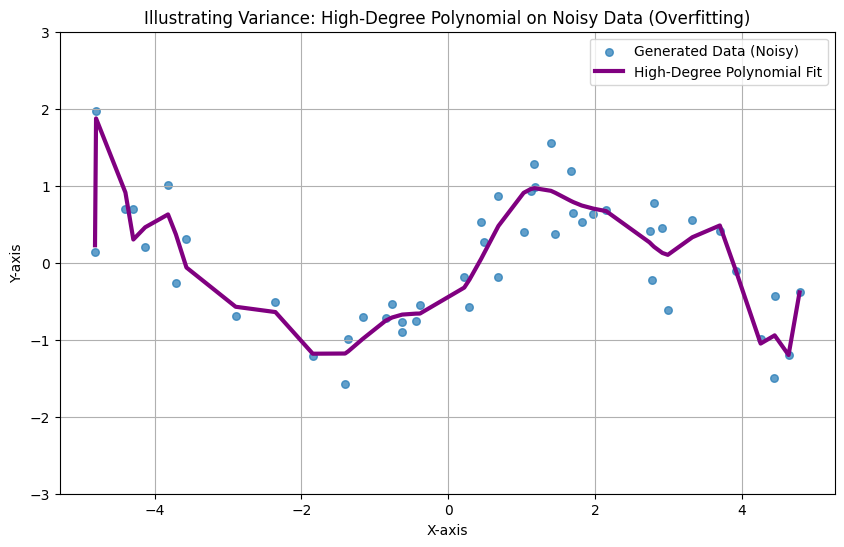
🛑 The Problem: High Variance & Overfitting
When a model is too complex (like a high-degree polynomial), it begins to “memorize” the noise and outliers in the training set rather than learning the underlying pattern. Mathematically, this manifests as exceptionally large coefficients (W).
Regularization solves this by adding a penalty term to our Loss Function (L). Instead of just minimizing the error, we now minimize:

1. Ridge Regression (L_2 Regularization)
Mathematical Foundation
Ridge Regression adds an L_2 penalty, which is the squared magnitude of the coefficients.

- lambda (Alpha): The hyperparameter that controls the penalty strength.
- Effect: It shrinks coefficients toward zero but never makes them exactly zero.
From-Scratch Implementation (Gradient Descent)
Using the logic from our repository, we implement the weight updates by taking the derivative of the loss function including the L_2 term.
Python
import numpy as np

class RidgeGD:
    def __init__(self, epochs=1000, learning_rate=0.01, alpha=1.0):
        self.learning_rate = learning_rate
        self.epochs = epochs
        self.alpha = alpha
        self.coef = None
        self.intercept = None

    def fit(self, X_train, y_train):
        self.coef = np.ones(X_train.shape[1])
        self.intercept = 0
        n = X_train.shape[0]

        for _ in range(self.epochs):
            y_hat = np.dot(X_train, self.coef) + self.intercept

            # Gradients with L2 Penalty
            intercept_der = -2 * np.mean(y_train - y_hat)
            coef_der = (-2 * np.dot((y_train - y_hat), X_train) / n) + (2 * self.alpha * self.coef)

            self.intercept -= self.learning_rate * intercept_der
            self.coef -= self.learning_rate * coef_der

    def predict(self, X_test):
        return np.dot(X_test, self.coef) + self.intercept
2. Lasso Regression (L_1 Regularization)
Mathematical Foundation
Lasso (Least Absolute Shrinkage and Selection Operator) uses an L_1 penalty — the absolute value of the coefficients.
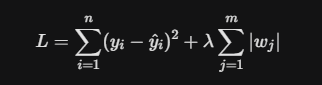
- The “Magic” of Lasso: Unlike Ridge, Lasso can drive unimportant feature coefficients to exactly zero.
- Use Case: This makes Lasso an excellent tool for Feature Selection.
From-Scratch Implementation
In our implementation, we use the np.sign() function to handle the derivative of the absolute value.
import numpy as np

class LassoRegressionGD:
    def __init__(self, lambda_=1.0, learning_rate=0.01, epochs=1000):
        self.lambda_ = lambda_
        self.learning_rate = learning_rate
        self.epochs = epochs
        self.coef = None
        self.intercept = None
        self.loss_history = []

    def fit(self, X_train, y_train):
        n_samples, n_features = X_train.shape
        self.coef = np.zeros(n_features)
        self.intercept = 0

        for epoch in range(self.epochs):
            y_hat = np.dot(X_train, self.coef) + self.intercept
            loss = np.mean((y_train - y_hat) ** 2) + self.lambda_ * np.sum(np.abs(self.coef))
            self.loss_history.append(loss)

            intercept_gradient = -2 * np.mean(y_train - y_hat)
            coef_gradient = -2 * np.dot(X_train.T, (y_train - y_hat)) / n_samples

            l1_penalty_gradient = self.lambda_ * np.sign(self.coef)
            coef_gradient += l1_penalty_gradient

            self.intercept -= self.learning_rate * intercept_gradient
            self.coef -= self.learning_rate * coef_gradient

    def predict(self, X_test):
        if self.coef is None:
            raise Exception("Model has not been fitted yet.")
        return np.dot(X_test, self.coef) + self.intercept

    def r2_score(self, y_true, y_pred):
        ss_total = np.sum((y_true - y_true.mean()) ** 2)
        ss_res = np.sum((y_true - y_pred) ** 2)
        return 1 - (ss_res / ss_total)
The Mathematical Secret: Why is Lasso Sparse?
Looking at your image, the red shapes represent the “budget” or constraint we give our coefficients (B1 and B2). The blue circles are the “loss contours” (where our model wants to go to fit the training data perfectly).

The “Solution” is the first point where the blue circles touch the red shape.
The Diamond vs. The Circle
- L1 (Lasso) Geometry: The constraint is a Diamond (|B1| + |B2| ≤ C). Because a diamond has sharp corners on the axes, the blue loss contours are mathematically much more likely to hit a corner first. At a corner, one of the coefficients is exactly zero.
- L2 (Ridge) Geometry: The constraint is a Circle (B1² + B2² ≤ C). A circle is smooth and has no corners. The loss contours will likely touch the circle at some point that is not on an axis, meaning both B1 and B2 stay alive, just smaller.
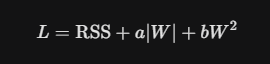
The Formulas
In your notes, you saw the “Total Error” formula. Regularization simply adds a penalty term to that error:

The (Lambda) is your “Tuning Knob.”
- A high lambda means you’re being very strict (High Bias, Low Variance).
- A low lambda means you’re letting the model be wild (Low Bias, High Variance).
3. Elastic Net: The Best of Both Worlds
When you have multiple correlated features, Lasso might arbitrarily pick one and ignore others. Elastic Net combines both L_1 and L_2 penalties to provide a balanced approach.
In practice, we use an l1_ratio to decide the balance between Ridge and Lasso.
The “Crucial Assumptions” Section
Before applying regularization, you must ensure your data meets these criteria:
- Feature Scaling (MANDATORY): Regularization penalizes the magnitude of coefficients. If one feature is in “kilometers” and another in “meters,” the penalty will be applied unfairly. Always use StandardScaler first.
- Linearity: The relationship between predictors and the target should still be linear.
- Independence of Errors: Ensure no autocorrelation in residuals.
🏆 Conclusion & Library Comparison
While our “from-scratch” NumPy models are great for understanding the math, industry tools like Scikit-Learn use more optimized solvers (like Coordinate Descent for Lasso). However, knowing the gradients and the penalty mechanics allows you to tune hyperparameters like alpha with intuition rather than guesswork.
What’s next? I’ll be diving into Feature Selection Techniques.
Let’s Connect!
- LinkedIn: pruthil-prajapati
- Email: Gmail
- GitHub: Pruthil-2910
Keep exploring the math behind the models!
#BuildInPublic #ArtificialIntelligence #DataEngineering #SoftwareEngineering #Mathematics #ProgrammingTips #100DaysOfCode #UnderTheHood #MathForML #FromScratch #CodeNewbie #Vectorization #Optimization #AlgorithmDesign #NumPy #Python
Behind the Scenes of Bias Variance Trade-Off and L1 , L2 Regularization was originally published in Towards AI on Medium, where people are continuing the conversation by highlighting and responding to this story.