
Agentic AI in Action — Part 16- The Data Warehouse That Built Itself: Powered by Snowflake CoCo
The Data Warehouse That Built Itself: Powered by Snowflake CoCo
How Snowflake’s Cortex Code (CoCo) turned plain English instructions into a fully working star-schema warehouse. No boilerplate, no hand-coded DDL.
There is a moment in every data engineering project where you stare at a blank SQL worksheet and think “I know exactly what this warehouse needs to look like. I just don’t want to type it”.
The schema is clear in your head. The transformations are obvious. You know you need a RAW layer for landing, a STAGE layer for cleaning, a FINAL layer for the star schema. But then you spend two hours constructing CREATE TABLE statements, wrestling with file format options you can never quite remember, and debugging a SPLIT_PART() and a LATERAL FLATTEN you last wrote ten months ago.
This blog is about skipping all of that. The warehouse we build is properly layered, analytically sound and is built describing each step in plain English to Snowflake’s Cortex Code assistant and letting it write the SQL.
Cortex Code (CoCo)
Cortex Code, which the community has taken to calling CoCo, is Snowflake’s AI powered coding agent that is available both within Snowsight (Snowflake’s UI) as well as in a CLI version. It is part of the broader Cortex AI suite and runs inside Snowflake Notebooks and SQL worksheets. CoCo uses a variety of advanced, large language models (LLMs), specifically designed for coding tasks.
We will be leveraging Cortex Code in Snowsight for this walkthrough. Cortex Code acts as an intelligent agent that translates your natural language instructions into executable actions. It stays aware of your workspace context and Snowflake account configuration, so you can handle development, exploration, and administration tasks, all without leaving Snowsight. Unlike a generic AI chat tool, CoCo is context-aware. It can see your database objects, your stage contents, and your existing tables.
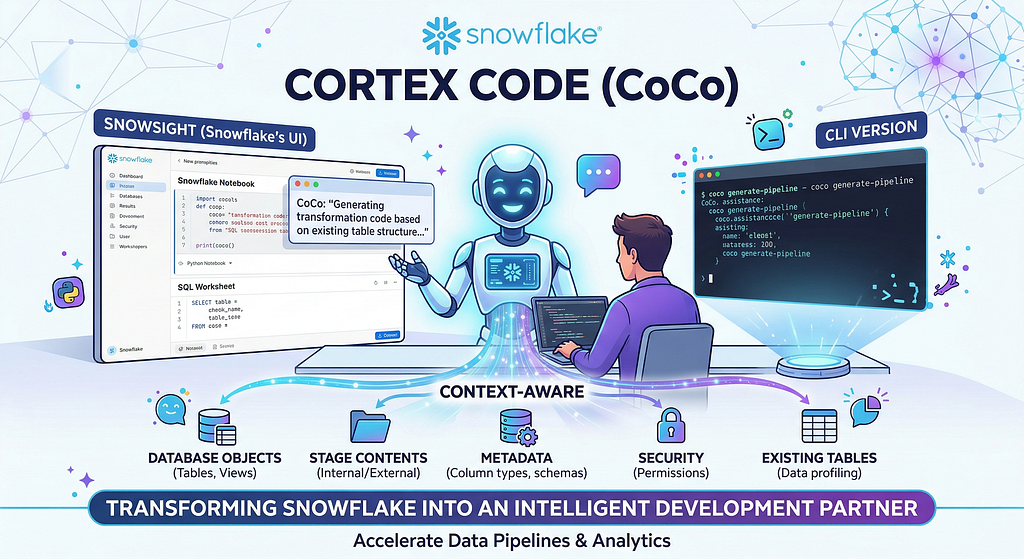
CoCo understands Snowflake’s metadata, security, and data structures to accelerate data pipeline development and analytics. When you describe a transformation, it already knows what columns exist and what the data looks like. In essence, CoCo transforms Snowflake from a data platform into an intelligent, context-aware development partner.
(Cortex Code is now generally available in Snowsight. The CLI version also offers native Windows support, enabling teams to use Cortex Code seamlessly in VS Code, Cursor, or any terminal of their choice. For detailed pricing information, please refer to the Cortex Code documentation here).
The Use Case:
This is best demonstrated through a practical, relatable use case. ShopFlash is a fictional e-commerce company that sells everything from wireless headphones to coffee makers. To keep things simple, we will work with three CSV files representing the core of ShopFlash’s business: Products, Customers, and Orders. By the end of this post, these files will have travelled through three schemas (RAW, STAGE, FINAL), cleaned, deduplicated, unpacked, and joined into a star schema, ready for analytics and reporting.

(A quick word on why we are starting with CSV files rather than a more sophisticated source like dbt models or a streaming pipeline. CSVs are the lowest common denominator in data engineering and they require no additional tooling to understand. They are also the easiest way to follow along. Download three files, upload them to a stage, and you are ready to go. In a real production setup you might land data from dbt models, Fivetran connectors, or event streams, and CoCo works just as naturally with any of those. But for a walkthrough focused on what CoCo can do, the simpler the source, the clearer the story and keeps things approachable for anyone exploring CoCo for the first time).
High-Level Architecture
ShopFlash’s warehouse will have three schemas.
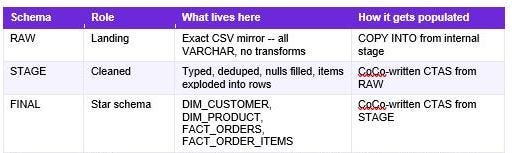
RAW is the landing zone. An exact mirror of the source CSV files, all VARCHAR columns, no transformations applied.
STAGE is the cleaning layer or the Refined layer. Proper types, nulls handled, emails normalized, and crucially the embedded line-item data in the orders file exploded into individual rows to create a new line items table.
FINAL is the star schema. It is the Curated layer. Dimension tables for customers and products, fact tables for orders and order line items, everything joined and keyed correctly for analytics.
The data flows in one direction. CSV files on a stage into RAW, transformed into STAGE, assembled into the FINAL star schema.

Dataset Overview
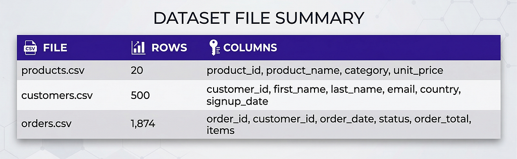
Here is a quick look at the three files that make up ShopFlash’s data. Understanding what’s in each one makes every transformation decision that follows feel obvious rather than arbitrary.
products.csv: 20 rows, one per product with name, category, and price. The smallest file but the backbone of every revenue-by-category query.
customers.csv: 500 rows of customer profiles. It has data quality issues (mixed-case emails and some blank country values) that the STAGE layer will clean up.
orders.csv: 1,874 rows, one per order. This is the most complex file because each row packs all its line items into a single pipe-delimited Items column that STAGE will unpack into individual rows.
What We Are Building
Before we write a single prompt, here is what we are building:
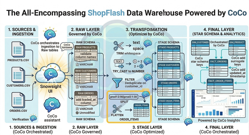
The diagram above shows the complete ShopFlash data pipeline that we will be building. Three layers, eleven tables, and one star schema, orchestrated entirely by CoCo. Raw CSV files flow in on the left, land in the RAW layer, get cleaned and unpacked in STAGE, and arrive in FINAL as analytics-ready dimension and fact tables. Do not worry if the elements in the diagram look like a lot right now. Every box, every arrow, and every transformation in it has its own dedicated step in the walkthrough ahead, and by the end, each one will feel completely natural.
Getting CoCo Ready
Before we jump into the implementation, let’s make sure everything is in place. It only takes a moment!

- Sign-up for a Snowflake Trial, if you don’t already have one.
- Ensure the following database roles are granted before proceeding: SNOWFLAKE.COPILOT_USER, along with either SNOWFLAKE.CORTEX_USER or SNOWFLAKE.CORTEX_AGENT_USER. If you are on a new trial account, these roles are already granted via your ACCOUNTADMIN privileges.
- Open a new SQL sheet in Snowsight
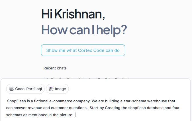
- Invoke Cortex Code from the right corner of your screen. You should then see a window similiar to the one below.

4. Rename to the SQL Sheet to something contextual. I called it “Coco-Part1”. You will see the name reflected in the dialogue box of cortex code window (as seen in the screen capture above)
5. Download the three csv files. customers.csv, products.csv and orders.csv, to your local machine. We will be uploading these to the internal stage in snowflake.
6. If Cortex functionality or specific models are not supported in your region, set Cross-Region Inference. For example, to allow ANY of the Snowflake regions that support cross-region inference to process your requests, you could run:
ALTER ACCOUNT SET CORTEX_ENABLED_CROSS_REGION = ‘ANY_REGION’;
Please review the documentation for additional details and cost information before enabling cross region inference.
7. Note that you could track CoCo spending using two specific account usage views: ACCOUNT_USAGE. CORTEX_CODE_CLI_USAGE_HISTORY for the CLI version and ACCOUNT_USAGE.CORTEX_CODE_SNOWSIGHT_USAGE_HISTORY for the Snowsight version (that we use for this walkthrough)
Now that we have the basics taken care of, let us begin talking to CoCo!
The step by step prompts and the files are available here.
The below steps would consist of a series of prompts and responses. (Please note that the responses you receive might slightly differ depending on the model choice as determined by CoCo at runtime).
The Complete ShopFlash walkthrough with Cortex Code

Step 1: Lay the Foundations
Every warehouse starts with a blank database. We will provide a context to CoCo and ask to create the SHOPFLASH database and its three schemas. The database and schema setup is shared with CoCo as a screenshot(see below) rather than typed out. This is a deliberate choice to showcase CoCo’s multimodal capability. It reads the image, understands the structure, and gets to work!
Prompt:
(Please attach the above image using the “+” option in the CoCo conversation wondow and enter the prompt below. The image is provided as part of the blog’s code files)
ShopFlash is a fictional e-commerce company. We are building a star-schema warehouse that can answer revenue and customer questions. Start by Creating the shopflash database and three schemas as mentioned in the picture.
You can observe the progress as the objects are created. A dialog box will ask you for a “Yes” before running each generated SQL, as shown below.
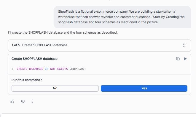
CoCo confirms that the database and the three schemas were created successfully:

Let us confirm this in the Snowsight UI as well:

Step 2: Creating an internal stage for the Landing zone
Before any data can enter Snowflake, it needs somewhere to land. Stage in Snowflake is a managed storage location that sits between your local files and your database tables. Think of it as an arrivals terminal at an airport. Data checks in here before being processed and sent to its final destination.
An internal stage is fully managed by Snowflake. No S3 bucket, no cloud credentials to configure. We will ask CoCo to create one with the right CSV settings baked in as a named file format:
The Prompt: In the SHOPFLASH database, create a named internal stage called SHOPFLASH_STAGE inside the RAW schema. Configure it for CSV files: comma-delimited, header row skipped, fields optionally quoted, and empty strings or the word NULL treated as SQL NULL.
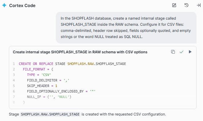
Those file format options mentioned in the prompt are important. FIELD_OPTIONALLY_ENCLOSED_BY handles product names that contain commas (“Coffee Maker, Large”). NULL_IF maps both blank strings and the literal text ‘NULL’ to a proper SQL NULL, which prevents silent data quality issues from propagating downstream.
Step 3: Upload the CSV files through Snowsight
With the stage created, we now upload the three CSV files directly through Snowsight by navigating to the stage and using the Upload Files button. This is the simplest path for files on your local machine, and it requires no command-line tooling. Browse and choose all three files. Select the schema (SHOPFLASH.RAW) and the newly created Stage (SHOPFLASH_STAGE). Click Upload.

Step 4: Let CoCo read the file and create RAW.PRODUCTS table
Here is where the workflow gets interesting. Rather than designing the RAW schema upfront, we pointed CoCo at the staged file and asked it to figure out the columns itself using INFER_SCHEMA (a Snowflake function that reads a file on a stage and returns the column names and suggested types). Notice that all columns are VARCHAR. This is intentional and important. The RAW layer is an immutable archive of exactly what the source file contained.
We start with products.csv, the simplest file.
Prompt:
I have a CSV file called products.csv on the stage
@SHOPFLASH.RAW.SHOPFLASH_STAGE.
create a named file format if required.
Use INFER_SCHEMA to inspect it, then write a CREATE OR REPLACE TABLE
statement for SHOPFLASH.RAW.PRODUCTS that:
— mirrors the CSV columns exactly
— keeps all columns as VARCHAR (no type casting in RAW)
— adds a _loaded_at TIMESTAMP_NTZ column with DEFAULT CURRENT_TIMESTAMP()
— first row in the file is the header row with column names

Step 5: Load PRODUCTS data to the RAW layer
With the table structure in place, we ask CoCo to copy the rows from the file.
Prompt: Copy the rows from products.csv to RAW.PRODUCTS
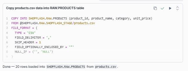
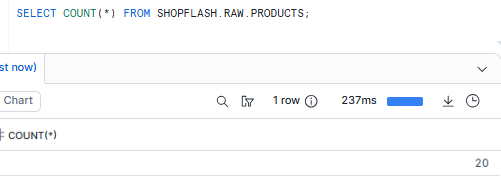
We will verify that the rows have been loaded successfully.
Step 6: Repeat the pattern for RAW.CUSTOMERS
For CUSTOMERS, we ask CoCo to follow the same pattern
Prompt: Similarly follow the same steps to copy customers.csv to RAW.CUSTOMERS. Follow the same approach that you just used for RAW.PRODUCTS.

Notice how CoCo retains the context from the previous steps and applied the same pattern to the new file. You are not rewriting instructions from scratch each time, you are building on a shared understanding, exactly the way you would with a colleague. The conversation is doing the work, not just the prompt.
500 customers loaded cleanly. The email column has mixed-case values and roughly 3% of rows have a blank country field.
Step 7: Repeat the pattern for RAW.ORDERS
Orders follows the same pattern for data loading, but with one thing worth pausing on-> The items column. In the source CSV, every order’s line items are packed into a single cell as a pipe-delimited string. For example “926897c2–7ac8–4fe9-af80–23019162863a:2:84.99|e2a9495d-7a2e-4252–8e17-ba650bf1a46c:3:54.99|7768e0b2-a3fe-4366-b313–3f2b9a7b2ba9:2:49.99|5656d8e6–2fbb-45fa-b907-e11cffa3cff1:3:24.99|a5a336c5–7a2d-4753-b3e5–42c7d9256692:1:129.99”
Each segment before a pipe represents one line item: product_id:quantity:unit_price. An order with five products has five colon-separated segments joined by pipes. In RAW we leave this entirely untouched with one row per order and the items string preserved as-is. The unpacking into individual rows happens in STAGE. (We will look at this closely during stage load).
Prompt: Similarly follow the same steps to copy orders.csv to RAW.ORDERS. Follow the same approach that you just used for the other two RAW tables

Let us validate the count and confirm that it loaded all the 1874 rows.

With that, we have successfully loaded all the tables to the RAW layer! Three tables, loaded without issues, every column VARCHAR, every row exactly as the source file sent it.
Step 8: Transforming RAW.PRODUCTS into STAGE
STAGE is where VARCHAR becomes NUMBER, whitespace gets trimmed, and null handling becomes explicit. For products, the transformations are simple. Trim trailing spaces from text columns and safely cast unit_price to a numeric type.
Prompt: Read from SHOPFLASH.RAW.PRODUCTS and create SHOPFLASH.STAGE.PRODUCTS.
Transformations needed:
— TRIM whitespace from product_name and category
— Cast unit_price from VARCHAR to NUMBER(10,2) using TRY_CAST
so bad values become NULL rather than erroring
— Drop rows where product_id is NULL
Note: TRY_CAST is the safe version of CAST. Where CAST throws an error if a value cannot be converted (crashing the whole query), TRY_CAST returns NULL instead. For warehouse work, TRY_CAST is almost always the right choice in STAGE. Bad values become NULL and are visible for investigation, rather than aborting the table creation entirely. You could choose to use strict CAST only in the FINAL layer, after you have confirmed STAGE contains no malformed values.
The product_id IS NOT NULL clause acts as a lightweight data contract where rows without an identifier are meaningless downstream and dropped early rather than silently propagating into FINAL.

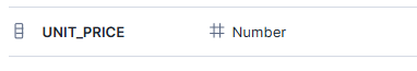
We can query the table and observe that the white spaces are trimmed in the product name and category fields. The unit_price is successfully convered to a numeric field.
Step 9: Transforming RAW.CUSTOMERS into STAGE
Customers need more work. Email normalization, null country handling, and deduplication. We describe all transformations in a single CoCo prompt:
Prompt: Read from SHOPFLASH.RAW.CUSTOMERS and create SHOPFLASH.STAGE.CUSTOMERS.
Transformations needed:
— normalize email to lowercase
— fill blank or null country with ‘Unknown’
— Deduplicate on customer_id, keeping the row with the latest _loaded_at
— Drop rows where customer_id is NULL
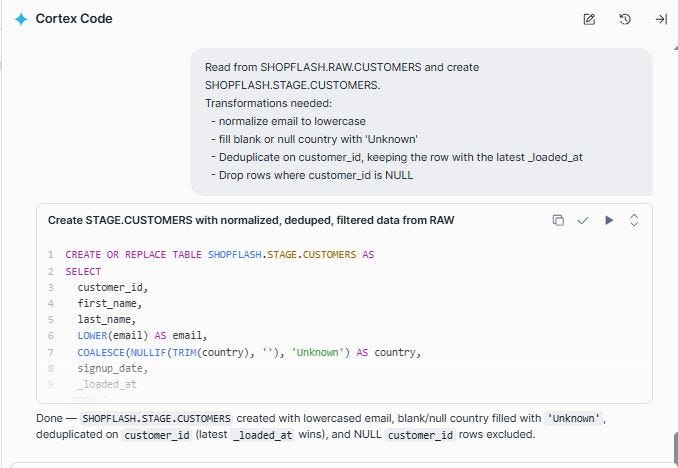
After running this, every customer_id is unique, every email is lowercase, and no country is blank. The data quality issues that arrived in RAW are fully resolved in STAGE.
Let us look at a sample row to confirm that the emails are in lower case and the blank or null country values are replaced with “Unknown”.

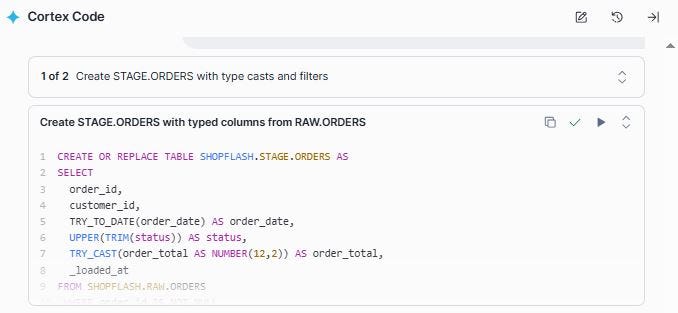
Step 10: Unpacking RAW.ORDERS to line items and load to STAGE
This is the most technically involved step in the whole pipeline, and the one where CoCo saved the most time. The orders file stores line items as a pipe-delimited string inside a single column. To do anything analytically useful, such as revenue by product, units sold per category etc., we need to unpack that string into individual rows with one row per order per product.
We describe exactly what we wanted and let CoCo figure out the Snowflake syntax. We will first provide the instructions for ORDERS and then the ORDER_ITEMS instructions to split and flatten.
Prompt: Read from SHOPFLASH.RAW.ORDERS and create two STAGE tables:
1. SHOPFLASH.STAGE.ORDERS
— TRY_TO_DATE(order_date)
— UPPER(TRIM(status))
— TRY_CAST(order_total AS NUMBER(12,2))
— Drop rows where order_id is NULL
2. SHOPFLASH.STAGE.ORDER_ITEMS
The ‘items’ column contains pipe-delimited strings, each in the
format ‘product_id:quantity:unit_price’.
Use LATERAL FLATTEN + SPLIT to explode one row per line item.
Calculate line_total = quantity * unit_price.
Generate a UUID for order_item_id using UUID_STRING().
CoCo completes this task sequentially as shown in the two screen shots below and creates the two tables successfully.

Let us look at this closely.
UUID_STRING(): Generates a universally unique identifier (UUID) — a random 36-character string. Because order items did not exist as separate records in the source file, they have no natural ID. UUID_STRING() gives each exploded line item its own stable, unique key.
LATERAL FLATTEN turns one row with five packed items into five rows. It is Snowflake’s way of unzipping compressed data.
SPLIT_PART(f.value::STRING, ‘:’, 1): Splits a string on a delimiter and returns the Nth segment. Consider the value ‘5656d8e6–2fbb-45fa-b907-e11cffa3cff1:3:24.99’, position 1 returns the product_id (abc123), position 2 the quantity(2), position 3 the unit_price(84.99). The ::STRING cast converts the VARIANT type that FLATTEN returns into text before splitting.
The pipe | separates products, and the colon : separates the fields within each product. So, multiple products are split from the same row into multiple rows, along with their corresponding quantity and price. SPLIT and LATERAL FLATTEN work together to unpack this. SPLIT breaks on the pipe to isolate each product segment, and SPLIT_PART then extracts position 1, 2, or 3 from each segment to get the individual field values.
We can query the table to examine this, along with the LINE_TOTAL that CoCo just created for us based on our prompt (as unit_price * quantity)
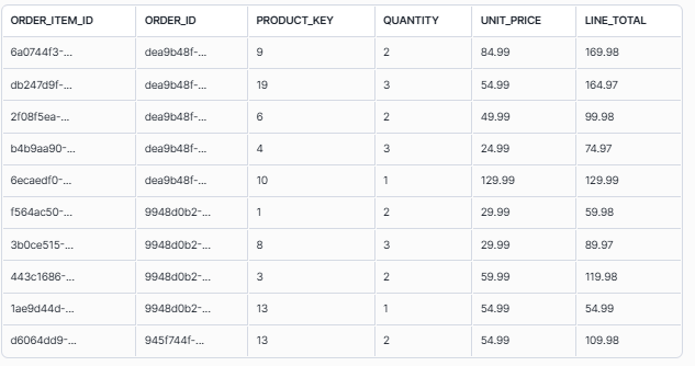
The result is 5634 rows in STAGE.ORDER_ITEMS from 1,874 orders, confirming that the LATERAL FLATTEN successfully unpacked each order’s line items into individual rows. We went from one packed column to a proper relational table with a row for every product on every order.

What even a seasoned engineer would double-check the documentation for, CoCo produced in a single prompt, on the first try!
Step 11: The checkpoint to confirm STAGE row counts
Before building FINAL on top of STAGE, it is worth pausing to confirm the numbers make sense. We will ask CoCo for a simple count across all four STAGE tables:

We are now ready to build the FINAL layer!
Step 12: Build the dimension tables in the FINAL layer
The FINAL schema is where data becomes analytics-ready. It follows the star schema pattern. Dimension tables describe the ‘who’ and ‘what’ (customers, products), and fact tables capture the ‘metrics’ (orders, order line items). Analytical tools, BI dashboards, SQL queries, ML models etc query FINAL DW layer. They never need to touch RAW or STAGE.
We start with the two dimension tables:
Prompt: From SHOPFLASH.STAGE, create two dimension tables in SHOPFLASH.FINAL:
1. FINAL.DIM_CUSTOMER
— All columns from STAGE.CUSTOMERS
— Add customer_key as a surrogate key using ROW_NUMBER()
ordered by signup_date, customer_id
— Add updated_at = CURRENT_TIMESTAMP()
2. FINAL.DIM_PRODUCT
— All columns from STAGE.PRODUCTS
— Add product_key as a surrogate key using ROW_NUMBER()
ordered by product_id
— Add updated_at = CURRENT_TIMESTAMP()
Note: Surrogate Key is a warehouse-generated integer separate from the source system’s business ID and is a common practice in Data warehouses. FACT tables join to DIM tables on these keys rather than raw UUIDs, because source IDs can change through migrations or re-registrations, while the surrogate key stays stable inside the warehouse no matter what happens upstream. Additionally, the updated_at column records when each DIM row was last written. If and when we move to incremental loads, updating FINAL only with rows that changed since the last run, this timestamp becomes the mechanism for detecting which records need updating.

Step 13: Complete the star schema with the FACT tables
FACT tables record events: an order was placed, a product was purchased. Each row in a fact table links to the relevant dimension records via their surrogate keys. The join happens here, in the FINAL load.
Prompt: From SHOPFLASH.STAGE, create two fact tables in SHOPFLASH.FINAL.
Join to the DIM tables already in FINAL to resolve surrogate keys:
1. FINAL.FACT_ORDERS
— From STAGE.ORDERS joined to FINAL.DIM_CUSTOMER on customer_id
— Include: order_id, customer_key, order_date, status, order_total
2. FINAL.FACT_ORDER_ITEMS
— From STAGE.ORDER_ITEMS joined to FINAL.FACT_ORDERS on order_id
and FINAL.DIM_PRODUCT on product_id
— Include: order_item_id, order_id, product_key,
quantity, unit_price, line_total

Let us preview the FACT_ORDER_ITEMS table

Step 14: From raw files to revenue figures. The final check!
Let us first ask CoCo to confirm the row counts in the FINAL layer
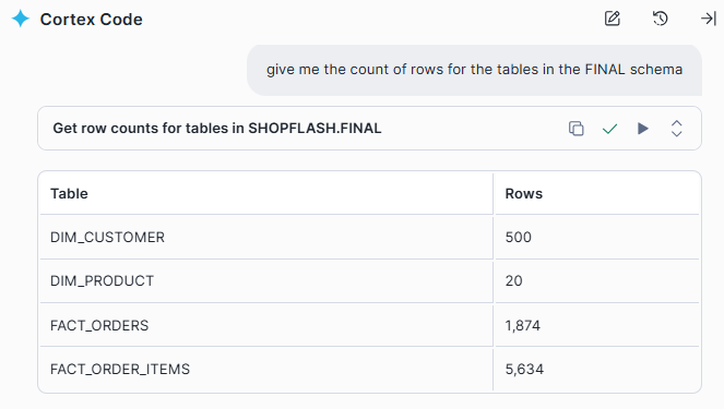
With FINAL populated, we ask CoCo for two analytical queries to confirm the star schema works end-to-end:
Prompt 1 : Give me the Total orders, total revenue, and average order value for completed orders

Prompt 2: Top 5 product categories by revenue

CoCo did not just write the query. It figured out which tables to join. Knowing that product category lives in DIM_PRODUCT and revenue lives in FACT_ORDER_ITEMS, it connected the two without being told, and surfaced the top five categories by revenue in a single shot.
And just like that, the warehouse is alive!
It is now ready to power dashboards, answer business questions, and feed machine learning models.
Fourteen steps ago, we had three CSV files and a Snowflake account. Now we have a fully layered, analytics-ready star schema with raw data preserved as an audit log, a clean STAGE with quality issues resolved, and a FINAL layer that can answer real business questions with a single SQL query.

This was a deliberately simple warehouse. No incremental loads, no versioned history etc. The goal of this walkthrough was to simply show how naturally data can travel from a raw file on a stage all the way to a queryable star schema, with CoCo guiding every step of the way. In a real production warehouse there is more to explore, and CoCo can take you there just as easily. SCD Type 2 to version customer records over time, incremental loads to process only what changed since the last run, data quality checks between layers to catch bad data before it reaches FINAL, clustering keys for faster time-range queries as the table grows etc. The pattern scales as far as your requirements do. You just keep describing.
But the more interesting story is what we did not do. We did not spend time wrestling with syntax. We did not puzzle over how to unpack a delimited column into rows. We did not hand-craft deduplication logic or figure out the right COALESCE pattern for null handling. We described our intent, reviewed what came back, and moved on.
That is the shift CoCo represents. Not replacing the engineer, but eliminating the gap between knowing what needs to be done and being able to express it in code.

The decisions were still ours. Which columns to clean, how to treat null codes, how to model the line items. We expressed the intent. CoCo wrote the code. And that coordination, with judgment and decisions on one side, execution and speed on the other, is exactly the point. Data engineers do not become obsolete with CoCo. They become unstoppable. The skill does not go away, the friction does.
The step-wise prompts and the associated data files can be accessed here.
I share hands-on, implementation-focused perspectives on Generative & Agentic AI, LLMs, Snowflake and Cortex AI, translating advanced capabilities into practical, real-world analytics use cases. Do follow me on LinkedIn and Medium for more such insights.
Agentic AI in Action — Part 16- The Data Warehouse That Built Itself: Powered by Snowflake CoCo was originally published in Towards AI on Medium, where people are continuing the conversation by highlighting and responding to this story.