Train Your Own AI Image Detector: Why Off-the-Shelf Detectors Fail on Your Data (DINOv2 + ConvNeXt…

Train Your Own AI Image Detector: Why Off-the-Shelf Detectors Fail on Your Data (DINOv2 + ConvNeXt, No GPU)

Off-the-shelf AI image detectors are everywhere — but that never seems to work for our own use case.

Companion to How I Distilled a Gemini Vision Model into a 4.6M-Parameter Model. Last time, the lesson was: you don’t need to fine-tune a backbone — freeze a big model, train a tiny head, ship it. This time I needed the backbone. The reason is the whole point.

Three numbers

A fashion-discovery feed is only as good as its images. And a growing share of what people upload now isn’t a photo of a real outfit — it’s an AI render. Some of it is stunning. Most of it is slop: plastic skin, six-fingered hands, a dress that ignores gravity. Left alone, it rots the feed.

The job: detect AI-generated images so we can filter them.

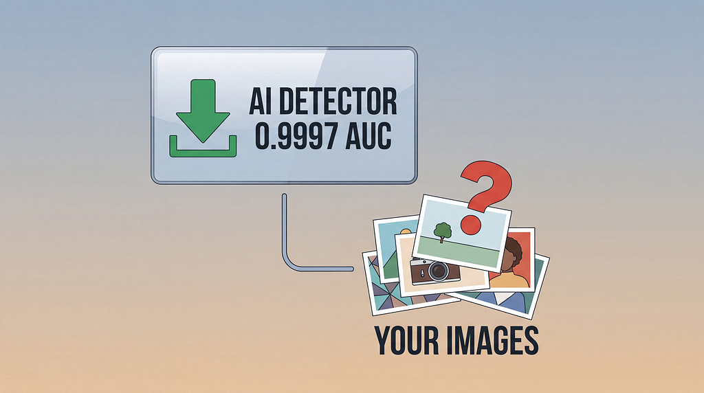
My first instinct was the lazy one — yours probably is too: someone has already built this AI image detector. And they have, dozens of times. Hugging Face is full of “AI vs. human” detectors you can download and self-host this afternoon, and the brochures are glorious. One recent detector reports a 0.9997 AUC on its validation set. Near-perfect.

So I downloaded a popular one and measured how well it agreed with the AI-probability labels we already trust in production. That measurement is the first snippet — and it’s the one that set the whole project in motion:

from transformers import pipeline
from sklearn.metrics import roc_auc_score
# a popular off-the-shelf detector - downloaded and run locally
clf = pipeline("image-classification", model="Organika/sdxl-detector", device="mps")
def p_ai(path):                       # the detector's probability that an image is AI
    out = {d["label"]: d["score"] for d in clf(path)}
    return out["artificial"]
preds  = [p_ai(p) for p in sample_paths]
y_true = [s >= 0.5 for s in teacher_ai_score]     # our production labels
print(roc_auc_score(y_true, preds))               # 0.68 - on *our* images

It scored 0.68. A throwaway linear model I’d wire up in the next section scored 0.82.

Three numbers — 0.9997, 0.68, 0.82. The first is what the shelf advertises. The second is what a real, published detector did on our data. The third is a ten-minute warm-up beating it. The whole article lives in that gap, and it isn’t a story about one bad model.

Why off-the-shelf AI-image detectors fail (it’s not bad luck)

This is a structural limit the research community keeps shouting about, and almost nobody building products hears.

AI-generated image detection is not solved. At ICLR 2025, a paper bluntly titled A Sanity Check for AI-Generated Image Detection built a deliberately hard benchmark and found that almost every off-the-shelf detector misclassifies AI-generated images as real the moment you leave its training distribution. A 2026 study of 16 detectors across 12 datasets found the same shape every time: gorgeous numbers in-distribution, a cliff outside it.

There are two cliffs.

Cross-generator. Train a detector on GAN images and it falls apart on diffusion images — each generator family leaves a different fingerprint. You’re always detecting yesterday’s fakes.

Cross-objective — the one that got me. My detector wasn’t asked “is this AI?” in the abstract. It was asked to agree with the specific AI-scores we run in production, on our image distribution — Pinterest-style fashion, not whatever set the downloaded model grew up on. Different target, different data, same word “fake” meaning two different things.

No download fixes that. The signal lives in your data, so you have to train on your data — which sounds expensive, right up until it isn’t.

A 20-second detour: where the signal hides

Generators build images by upsampling — doubling resolution again and again to fill in detail. That leaves faint, regular fingerprints in the frequency domain near the high-frequency edges of the image: periodic patterns your eye never registers but a model can (Frank et al., ICML 2020; Durall et al., CVPR 2020; CNNSpot, CVPR 2020). Detection isn’t about content — “is this a plausible dress?” It’s about texture statistics: the microscopic signature of how the pixels were synthesized.

Hold that thought. It’s why the cheap trick almost worked — and why it didn’t quite.

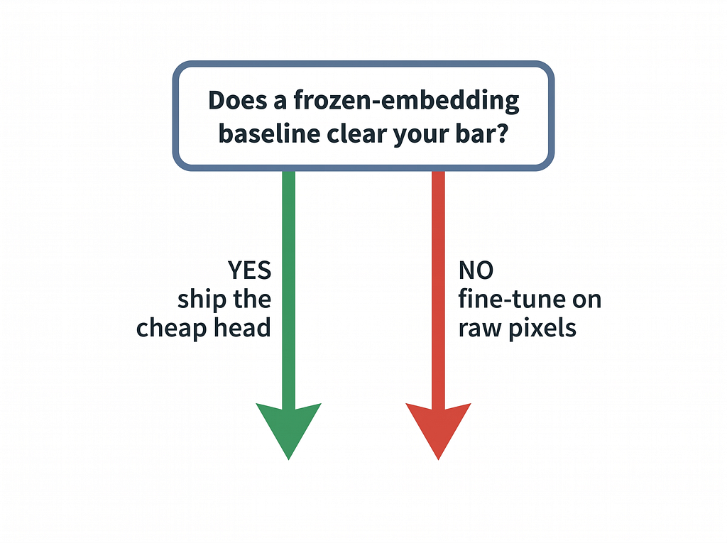
Attempt 1: a frozen DINOv2 baseline (it gets you 80% of the way)

In my last piece, the move was: don’t train a vision model — freeze a big one, grab its embeddings, train a tiny head. So I tried it here: every image through DINOv2 (Meta’s self-supervised ViT) → a 768-dim embedding → a dead-simple logistic regression. No fine-tuning yet — just a frozen DINOv2 feature extractor and a linear probe.

import timm, torch
from sklearn.linear_model import LogisticRegression
from sklearn.preprocessing import StandardScaler
dino = timm.create_model("vit_base_patch14_dinov2.lvd142m",
                         pretrained=True, num_classes=0).eval()   # frozen - pure inference
@torch.no_grad()
def embed(batch):                       # batch: (N, 3, 224, 224)
    return dino(batch).cpu().numpy()    # (N, 768)
# X = DINOv2 embeddings for ~36k images; y = (teacher_ai_score >= 0.5)
Xs = StandardScaler().fit_transform(X)
probe = LogisticRegression(max_iter=2000, class_weight="balanced").fit(Xs, y)

0.82 ROC-AUC. From a linear model. No fine-tuning, no GPU, a few seconds of training.

And here’s where the lazy hot-take (“frozen embeddings are useless for detection”) is just wrong: that 0.82 isn’t a failure — it’s a strong, free baseline, and the literature predicted it. UnivFD (CVPR 2023) showed a linear classifier on frozen CLIP features out-generalizes CNNs trained from scratch. And recent forensics work found DINOv2 is especially good here — its self-supervised features preserve fine-grained texture better than CLIP’s semantic ones, so a linear head on DINOv2 can beat fully supervised models.

The frozen DINOv2 baseline got me most of the way for free. The only question left: is the last mile worth it?

Before training: look at your labels

Before fine-tuning anything, I looked at the label distribution. This is the snippet I run on every new dataset, and it saved me an afternoon of chasing the wrong fix:

import pandas as pd
labels = pd.read_parquet("labels.parquet")          # one row/image: ai_score in [0, 1]
print((labels.ai_score < 0.1).mean())               # 0.75  -> 3 in 4 are obviously "real"
print((labels.ai_score >= 0.5).mean())              # 0.11  -> only ~11% are "likely AI"

Three out of four images sat near zero; only ~11% were “likely AI.” I wrote “will need class weighting” in my notes before training a thing. Remember that — it’s the plot twist.

Attempt 2: fine-tuning ConvNeXt to detect AI images (the last mile, on raw pixels)

The frozen DINOv2 probe plateaued at 0.82 because a frozen backbone only hands you the signal it already encodes. To surface this teacher’s artifacts, the model has to see raw pixels and adapt its own low-level filters. So I fine-tuned a small CNN end-to-end — ConvNeXt-Tiny (not a random pick: a strong ICLR 2025 detector, AIDE, is also ConvNeXt-based).

Three choices mattered, and every one is backwards from normal image classification. The first one is a custom transform, and it’s the most important line in the whole project:

import random
from PIL import Image
class NativeCrop:
    """Take a 224px square at NATIVE resolution. NEVER downscale - that smears the high-frequency
    artifacts we're trying to detect. Only upscale when the image is smaller than the crop."""
    def __init__(self, size=224, train=True):
        self.size, self.train = size, train
    def __call__(self, img: Image.Image) -> Image.Image:
        w, h, s = *img.size, self.size
        if min(w, h) < s:                                   # too small -> upscale just enough
            scale = s / min(w, h)
            img = img.resize((round(w * scale), round(h * scale))); w, h = img.size
        left = random.randint(0, w - s) if self.train else (w - s) // 2
        top  = random.randint(0, h - s) if self.train else (h - s) // 2
        return img.crop((left, top, left + s, top + s))

The other two choices:

• Almost no augmentation. The usual bag — blur, JPEG, color jitter — destroys or fakes the exact artifacts that mark an image as synthetic. Horizontal flip and nothing else.
• Full fine-tune. Don’t freeze the early layers. Normal transfer learning freezes the stem. Here it’s the opposite: the artifacts live in the early conv filters, so those are exactly the ones that have to move.

Now the model, the loss, and the training step. The loss is where the plot twist pays off:

import timm, torch, torch.nn as nn
model = timm.create_model("convnext_tiny", pretrained=True, num_classes=1).to("mps")
# soft-label distillation: BCE against the teacher's 0–1 score.
# pos_weight counters the ~11%-positive imbalance we found above.
pos_weight = torch.tensor((1 - y.mean()) / y.mean())      # ≈ 6
loss_fn = nn.BCEWithLogitsLoss(pos_weight=pos_weight)
opt = torch.optim.AdamW(model.parameters(), lr=1e-4, weight_decay=0.05)
for x, target in loader:                                  # target = teacher's soft 0–1 score
    with torch.autocast("mps", dtype=torch.bfloat16):
        loss = loss_fn(model(x.to("mps")).squeeze(1), target.to("mps"))
    opt.zero_grad(); loss.backward(); opt.step()

The one line that mattered more than the architecture

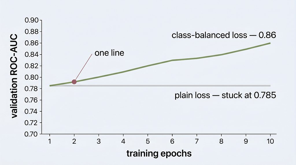
Here’s the twist I set up earlier. My first fine-tune used a plain loss — no pos_weight — as a baseline. It did exactly what an imbalanced dataset makes a model do: it plateaued at 0.785. Below the free probe. With a plain loss, the model found the cheapest possible strategy — call everything “real,” eat the 11% error, go home. Low loss. Useless detector.

The fix wasn’t a bigger model or more epochs. It was the pos_weight ≈ 6 you already saw — one line — so the rare AI images actually pulled on the gradient. That single change broke the plateau and the model climbed to 0.86 validation, 0.84–0.875 on the held-out test set.

Same model. Same data. One line.

When a model stalls, suspect the loss and the data before you touch the architecture. I keep relearning this, and I keep writing it down so maybe one day I’ll learn it.

Did it actually learn — or just memorize?

A detector that nails the training set and flops in production is worse than useless. So the last snippet is the one that earns trust: the held-out evaluation, reported the way an imbalanced problem demands — ROC-AUC and PR-AUC, not accuracy (with ~11% positives, “always predict real” scores 89% accuracy and catches zero fakes).

from sklearn.metrics import roc_auc_score, average_precision_score
@torch.no_grad()
def evaluate(model, loader):
    p, y = [], []
    for x, target in loader:
        p += torch.sigmoid(model(x.to("mps")).squeeze(1)).cpu().tolist()
        y += target.tolist()
    yb = [t >= 0.5 for t in y]
    return roc_auc_score(yb, p), average_precision_score(yb, p)
# train-sample vs held-out test: gap ≈ 0.035 -> generalizing, not memorizing
print(evaluate(model, test_loader))     # (0.843, ...)

The train-vs-test ROC gap came out to ≈ 0.035 — basically nothing. It generalized.

What I shipped

A ConvNeXt-Tiny AI-image detector, fine-tuned end-to-end, agreeing with our production AI-scores at ~0.84–0.875 ROC-AUC. The payoff still feels slightly illegal:

• It trained on a MacBook. No cloud GPU, no cluster — minutes per epoch on the laptop’s Apple GPU.
• Inference is effectively free — a small CNN, milliseconds an image, zero per-call API bill.
• We own it. It runs in our pipeline, on our distribution, tuned to our definition of “fake.”

The detector I couldn’t download, I trained over an afternoon for the price of some electricity.

The honest part

Three caveats, said out loud so you don’t have to find them:

• Frozen features didn’t fail. They got 80% of the way for free; for plenty of teams that’s the finish line. Fine-tuning bought a modest last mile, not a miracle.
• I’m distilling a teacher, not discovering truth. The model agrees with our AI-scores and inherits their blind spots. It can’t beat what taught it.
• You maintain this, you don’t ship-and-forget it. New generators leave new fingerprints; every detector decays (ICLR 2025).

The takeaway

When you need a model, the reflex is to go shopping. For AI-generated image detection the shelf is full — and most of it won’t fit your data. That’s not bad luck; it’s the documented generalization gap, and it’s the title of this article.

But the reflex hides the real lesson: training your own AI image detector stopped being the expensive option. A frozen foundation model hands you a strong baseline for free; a few minutes of fine-tuning on a laptop closes the gap. You don’t need the GPU cluster you were dreading. You need the right loss, native-resolution crops, and the nerve to close the download tab and open a notebook.

Last time I told you that you don’t need to fine-tune a backbone. This time I did — and now you can tell which room you’re standing in.

The detector you can download was trained on someone else’s images. Yours weren’t.

If you’ve built a model that had to survive contact with real, messy, in-the wild data — what broke? I read every reply.

---

Train Your Own AI Image Detector: Why Off-the-Shelf Detectors Fail on Your Data (DINOv2 + ConvNeXt… was originally published in Towards AI on Medium, where people are continuing the conversation by highlighting and responding to this story.