LLM Quantization, Kernels, and Deployment: How to Fine-Tune Correctly, Part 5

digitado ⋅ 1 de April de 2026

The Unsloth deep dive into GPTQ, AWQ, GGUF, inference kernels, and deployment routing

A 1.5B model quantized to 4-bit can lose enough fidelity that instruction-following collapses entirely. A GPTQ model calibrated on WikiText and deployed on domain-specific medical text silently degrades on exactly the inputs that matter most. A Mixture-of-Experts model budgeted for 5B active parameters actually needs VRAM for all 400B.

None of these failures produce error messages. All of them produce models that look fine on benchmarks and fail in production. The common thread is that the post-training pipeline, everything between the last training step and the first served request, was treated as a formatting step rather than an engineering problem.

This episode opens that pipeline. From the moment LoRA adapters get merged into base weights, through the mathematics of how GPTQ and AWQ decide which bits to keep, into the kernel-level engineering that determines whether quantization actually translates into speed, and finally into the deployment routing decisions that determine whether the model runs on a MacBook, a cloud GPU, or an H100 cluster. Every stage has its own failure modes. Every stage has parameters that interact with decisions made in the stages before and after it.

Episode 1 mapped the transformer’s internal structure. Episodes 2 through 4 covered LoRA mechanics, data engineering, and training hyperparameters. This episode covers what happens after training ends, and why most production failures live here, not in the training loop.

The Merged Checkpoint
Post-Training Quantization
The GGUF Ecosystem
Inference Kernels
VRAM Math
The Quantization Floor and QAT
Deployment Routing and Operational Survival

Chapter 1: The Merged Checkpoint

Your Only Source of Truth

Before a model can be quantized, exported, or deployed, it needs to exist as a single, complete set of weights. This chapter covers the merge step that produces that artifact, and the operational errors that corrupt it.

1.1 Why Merging Exists

A LoRA fine-tuning run does not modify the base model. It trains two small matrices, A and B, for each targeted layer, and the learned update is their product AB. During training, the base weights W stay frozen. The adapter contribution gets added at inference time.

This separation is useful during training. It is a liability during deployment. Serving a model with adapters applied at runtime means carrying two sets of weights, running the matrix multiplication for AB on every forward pass, and managing the adapter loading logic in the serving stack. For production, the adapter needs to disappear into the base model.

That is what merging does. Unsloth’s save_pretrained_merged function with the merged_16bit parameter takes each frozen weight tensor W and adds the corresponding LoRA product AB directly into it. The output is a single unified model in FP16 or BF16 precision, saved as safetensors files. No adapters. No runtime overhead. Just one complete set of weights.

This merged FP16 checkpoint is the canonical source of truth for every downstream optimization. Every GGUF export, every AWQ quantization, every GPTQ compression is a lossy transformation derived from this file. The quality ceiling for any quantized model is set here. No quantization format can recover information that was lost or corrupted at the merge stage.

1.2 What Goes Wrong

The merge step is conceptually simple, matrix addition, but operationally fragile in ways that cost real debugging hours.

Recursive merging in containers. In containerized environments, Unsloth may re-download the base model weights if the Hugging Face Hub cache is not correctly mapped to the container’s filesystem. When this happens, the downloaded weights can end up in a hidden .cache directory inside the output folder. If the output directory is not cleared between runs, a subsequent merge can pick up already-merged weights as the “base,” applying the LoRA adapters a second time. The result is a model with LoRA deltas applied twice, a corrupted weight distribution that produces subtly wrong outputs. Subtle enough that it might pass a quick sanity check. Wrong enough that downstream quantization amplifies the error into visible degradation.

OOM during the merge itself. Merging a large model requires holding both the base weights and the merged output in memory simultaneously. For 70B+ parameter models, this exceeds the VRAM budget of most single-GPU setups. The maximum_memory_usage parameter controls how much GPU memory Unsloth allocates during the merge operation. The default of 0.75 is often too aggressive for large models. Reducing it to 0.5 or lower forces the merge to proceed in smaller chunks, avoiding OOM at the cost of longer merge times.

The irreversibility principle. If a deployment target changes after quantization, or if a specific quantization level produces unacceptable quality loss, the correct recovery path is always back to the FP16 merged checkpoint, never forward from the quantized model. Re-quantizing an already quantized model compounds precision loss at every step. A practitioner who skips the explicit creation of a merged FP16 checkpoint, going directly from adapters to a 4-bit export, has no recovery path. The training run must be repeated, or the adapters must be re-merged from scratch.

The pattern here is worth internalizing. The merged FP16 file is small relative to the effort that produced it, typically a few hours of fine-tuning plus compute cost. But it is the single artifact that determines the upper bound of every model that gets served in production. Protecting its integrity, verifying the merge was clean, storing it before any quantization step, is not excessive caution. It is the minimum responsible workflow.

Chapter 2: Post-Training Quantization

Two Algorithms, Two Philosophies

The merged FP16 checkpoint is the starting point. This chapter covers the two dominant algorithms that compress it, GPTQ and AWQ, and why they make fundamentally different bets about what to preserve.

2.1 What Quantization Actually Does

Quantization reduces the numerical precision of model parameters. A weight stored as a 16-bit floating-point number occupies two bytes. The same weight stored as a 4-bit integer occupies half a byte. For a 7-billion parameter model, that difference translates from roughly 14GB of VRAM down to roughly 3.5GB. The model becomes servable on hardware that could not previously hold it.

The compression is lossy. Every weight that was a precise floating-point value becomes one of a small set of discrete integers. Information is destroyed. The question that separates quantization algorithms is not whether information is lost, but which information, and how the algorithm decides what to sacrifice.

Two algorithms dominate production quantization today. They start from the same FP16 merged checkpoint. They produce models at the same target bit-width. But they optimize for fundamentally different objectives, and that difference determines when each one is the right choice.

2.2 GPTQ: Hessian-Guided Compression

GPTQ is a one-shot weight quantization method built on approximate second-order information. The core idea is precise. For each layer in the model, GPTQ finds the set of quantized weights that minimizes the difference between the original layer’s output and the quantized layer’s output when both are applied to a calibration dataset. The objective function is “argmin ||WX − ŴX||²”, where W is the original weight matrix, Ŵ is the quantized version, and X is the calibration input.

The algorithm processes weights sequentially within each layer. When one weight is quantized, the rounding error it introduces is compensated by adjusting the remaining unquantized weights. This compensation is guided by the Hessian matrix, the second-order derivatives of the loss with respect to the weights. The Hessian tells the algorithm which weights are most sensitive to perturbation, allowing it to distribute rounding error toward weights where it causes the least damage.

Computing and inverting a full Hessian at the scale of 175 billion parameters is intractable. GPTQ handles this through Cholesky reformulation, which provides numerical stability and reduces the quantization process to a few hours on modern GPUs even for the largest models.

The approach comes with a specific vulnerability. GPTQ’s error compensation is entirely shaped by the calibration dataset X. The Hessian is computed with respect to that data. If a fine-tuned model, one trained on domain-specific medical text for example, is quantized using a generic calibration set like WikiText, the Hessian reflects the wrong distribution. The algorithm optimizes weight rounding for text it will never see in production, while potentially introducing larger errors on the text it will actually process. This is calibration overfitting, and it is the most common source of unexpected quality degradation in GPTQ-quantized models.

The practical implication is straightforward. GPTQ produces excellent results when the calibration data matches the deployment distribution. When it does not match, quality drops in ways that standard perplexity benchmarks on the calibration set will not reveal.

2.3 AWQ: Protecting What Matters

AWQ starts from a different observation entirely. Not all weights contribute equally to model quality. A small fraction of parameters, roughly 1%, are disproportionately responsible for preserving accuracy. AWQ calls these “salient” weights, and its entire strategy is built around protecting them during compression.

The insight that makes AWQ work is counterintuitive. The importance of a weight is not determined by the magnitude of the weight itself, but by the magnitude of the activations that flow through it. A weight might be numerically small, but if the activations it multiplies are consistently large, quantization error on that weight gets amplified through every forward pass. AWQ identifies these critical weights by running a small calibration set and collecting activation statistics across the network.

Once salient weights are identified, AWQ applies a per-channel scaling factor before quantization. The math is “Q(W × s) · (X / s) ≈ W · X”. The scaling factor s inflates the salient weights into a range where quantization preserves more of their precision, while the corresponding input is divided by s to keep the output mathematically equivalent. The algorithm performs a per-layer grid search for the optimal scaling factor, parameterized by an exponent α typically between 0.25 and 0.75, that minimizes output error.

The result is a model where every weight sits in a uniform 4-bit format. No mixed precision, no special handling at the hardware level. This uniformity matters for inference kernels, which can process all weights through the same execution path without branching.

AWQ’s calibration robustness is its most practically significant advantage over GPTQ. Because AWQ protects weights based on activation patterns rather than optimizing reconstruction error for a specific dataset, it generalizes better to out-of-distribution prompts. A model quantized with AWQ using a generic calibration set will typically retain more quality on unseen domains than the same model quantized with GPTQ using the same generic set.

The quantization process itself is also faster. Where GPTQ requires several hours for large models due to the Hessian computation and sequential weight processing, AWQ completes in minutes. The activation statistics collection is a single forward pass over a small calibration set, and the scaling factor search is computationally lightweight.

2.4 When to Use Which

The decision between GPTQ and AWQ is not about which algorithm is “better.” It is about which trade-off matches the deployment scenario.

GPTQ is the right choice when the calibration data can be made to match the production distribution precisely. If the model was fine-tuned for a specific task, and representative data from that task is available for calibration, GPTQ’s Hessian-guided optimization will squeeze maximum quality out of the target bit-width for that distribution. The cost is sensitivity. The model is optimized for exactly that distribution, and performance on anything outside it is not guaranteed.

AWQ is the right choice when the model will encounter varied or unpredictable inputs. API-serving scenarios where user prompts span arbitrary topics, general-purpose assistants, or any deployment where the input distribution cannot be tightly controlled. AWQ’s activation-aware scaling provides more stable quality across distributions, with faster quantization times as a secondary benefit.

Both algorithms produce weights that are, on their own, just numbers stored in a file. How those numbers get packaged and executed depends on the deployment target. For local and cross-platform deployment, that means the GGUF format. For GPU serving, it means inference kernels.

Chapter 3: The GGUF Ecosystem

Local Deployment’s Native Format

GPTQ and AWQ target GPU serving stacks. But a large and growing share of LLM deployment happens on laptops, Mac Studios, and ARM-based edge devices where those formats do not apply. This chapter covers GGUF, the format built for that world, and the quantization logic that makes it work.

3.1 What GGUF Is

GGUF [GGML Unified Format] is not just a weight format. It is a container. A single GGUF file packages the quantized model weights alongside the tokenizer configuration, the chat template, and hardware-specific metadata into one portable artifact. This is what makes it the standard for local and cross-platform deployment through inference engines like llama.cpp and Ollama.

The container design solves a practical problem that plagues other formats. A model exported as raw safetensors requires a separate tokenizer file, a separate chat template configuration, and manual setup in the inference engine. Each of those is a point of failure. GGUF eliminates the assembly step by embedding everything the inference engine needs into the model file itself. One file, one download, one load command.

The runtime targets for GGUF are fundamentally different from GPTQ and AWQ. Where those algorithms assume NVIDIA GPU execution with CUDA kernels, GGUF models run through llama.cpp’s inference engine, which supports CPU execution, Apple Silicon’s Metal framework, and ARM-based processors. The same GGUF file can run on a MacBook Pro, a Raspberry Pi, or a cloud CPU instance without modification.

3.2 K-Quantization: Mixed Precision at Block Level

Legacy quantization formats applied a uniform bit-width to every weight in the model. Every tensor got the same treatment regardless of its role in the network. K-quantization, the standard scheme within GGUF, rejects that uniformity.

K-quants apply mixed-precision logic at a block level, identifying critical tensors within the model and assigning them higher precision while compressing less sensitive tensors more aggressively. Half of the attention value projection (attention.wv) and the second feed-forward matrix (feed_forward.w2) are quantized at 6-bit precision, while the remaining weights are compressed to 4-bit. These specific tensors, the value projection and the FFN down projection, are historically the most sensitive to precision loss. Episode 1 covered why: the value projection carries the content that flows forward when an attention match occurs, and the down projection integrates the gated FFN output back into the residual stream. Losing precision on either one degrades the signal at the exact points where information consolidation happens.

The result of this selective treatment is measurable. K-quant models achieve lower perplexity scores than uniform 4-bit models at the same file size. The bits are allocated where they matter most.

3.3 Unsloth Dynamic 2.0

Standard K-quants use a fixed rule for which tensors receive higher precision. The Q4_K_M recipe is the same regardless of whether the model is a 7B general-purpose assistant or a 70B code generator. Unsloth’s Dynamic 2.0 quantization replaces that fixed rule with a data-driven one.

Dynamic 2.0 profiles every individual layer in the model, analyzing the weight distribution and activation variance to determine each layer’s sensitivity to compression. This profiling uses a hand-curated calibration dataset of 300K to 1.5 million tokens, depending on the model, spanning code, dialogue, and reasoning tasks. Layers that show high robustness to precision reduction get dropped to lower bit-widths. Layers that show high sensitivity are kept at higher precision.

The optimization target is also different from standard K-quants. Where traditional quantization often optimizes for perplexity, Dynamic 2.0 minimizes the KL divergence between the quantized model’s output distribution and the FP16 baseline’s output distribution. This distinction matters in practice. Perplexity measures the average prediction quality across a dataset. KL divergence measures how well the entire probability distribution is preserved at each prediction step. A model can have acceptable perplexity while still flipping individual answer choices because the probability mass shifted just enough at critical decision points. Minimizing KL divergence reduces these “flips” in answer correctness, which is a more faithful measure of whether the quantized model actually behaves like the original.

3.4 The Quality Tiers

GGUF quantization levels form a clear hierarchy of quality retention versus deployment target. A 8.5 bits per weight targets high-end machines with 48GB+ VRAM or well-equipped Macs. 6.6 bits per weight serves as the default for 7B to 14B models where quality matters. 5.5 bits per weight balances quality against VRAM on consumer hardware. 4.8 bits per weight targets consumer-grade 24GB GPUs. 4.4 bits per weight pushes aggressive compression for lightweight agents. The exact quality retention at each tier depends on the specific model, its architecture, and the task, but the general pattern is consistent: larger models tolerate lower bit-widths with less degradation than smaller ones. Chapter 6 covers that relationship in detail.

The right tier is not determined by “how much quality can I afford to lose.” It is determined by the VRAM budget remaining after accounting for the KV cache at the target context length. Chapter 5 covers that calculation in detail. But the principle is simple. Choosing Q6_K for a 14B model on a 24GB GPU looks reasonable until the context window extends to 32k tokens, at which point the KV cache consumes the headroom that the higher-quality quant assumed was available. The quantization level and the context length are a joint decision, not two independent ones.

Chapter 4: Inference Kernels

Where Speed Actually Comes From

Chapters 2 and 3 covered how quantization algorithms and formats decide which bits to keep. This chapter covers what happens after that decision is made, at the hardware level where quantized weights either translate into real throughput gains or do not.

4.1 The Kernel-Algorithm Separation

A quantized model sitting on disk is just a file of compressed numbers. The algorithm that produced those numbers, whether GPTQ or AWQ, determined their values. But values alone do not generate tokens. Something has to move those 4-bit weights from VRAM into the GPU’s compute units, unpack them, multiply them against activations, and write the results back. That something is the inference kernel.

This separation is the single most important concept in LLM deployment performance, and the one most frequently ignored. The algorithm and the kernel are independent choices. The same AWQ-quantized model, identical weights, identical file, can produce wildly different throughput depending on which kernel executes it. In benchmarks using vLLM on Qwen2.5–32B-Instruct with an H200 GPU, an AWQ model running without the Marlin kernel achieved 67 tokens per second. The same model with Marlin achieved 741 tokens per second. A 10.9x difference. Same weights. Same hardware. Different kernel.

That number should be uncomfortable. It means a team can spend weeks optimizing their quantization pipeline, carefully selecting calibration data, tuning GPTQ’s Hessian computation or AWQ’s scaling factors, and then lose an order of magnitude of potential throughput by defaulting to whatever kernel their serving framework happens to load.

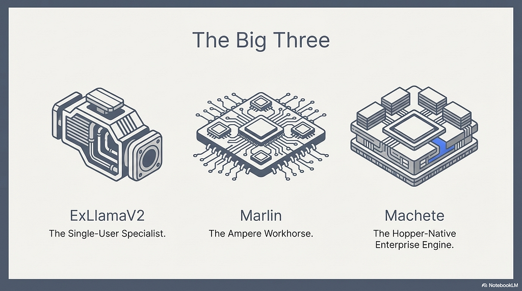
4.2 Marlin: The Ampere Workhorse

LLM inference at small batch sizes is memory-bandwidth bound: the GPU spends more time moving weights from global memory than performing matrix multiplications. Quantization helps by reducing memory traffic, but naive 4-bit implementations lose their advantage at larger batch sizes because they require explicit dequantization of weights back to FP16, introducing significant compute overhead.

Marlin addresses this by fusing dequantization directly into the matrix multiplication. Instead of converting INT4 weights to FP16 beforehand, Marlin performs computations on quantized weights directly within tensor core operations, eliminating the separate dequantization step and preserving the memory-bandwidth advantage even as batch size increases.

To further improve efficiency, Marlin uses asynchronous global memory loads that stream weights directly into shared memory, bypassing the L1 cache. This avoids cache pollution and enables overlap between memory transfers and computation, while one tile is being processed, the next is already being loaded.

Additionally, Marlin arranges quantized weights in memory layouts that align with tensor core tile requirements. This eliminates costly data reordering in registers and reduces register pressure, improving warp occupancy and overall throughput.

Together, these optimizations allow Marlin to achieve up to ~3.9× speedups over FP16 inference on NVIDIA Ampere and Ada GPUs (e.g., A100 and RTX 30/40 series), particularly for batch sizes up to 16–32.

4.3 Machete: Hopper-Native

Hardware evolves. Kernels optimized for one GPU generation do not automatically extract peak performance from the next. The Machete kernel is Marlin’s successor, designed specifically for the NVIDIA Hopper architecture and the H100 GPU.

Machete is built on CUTLASS 3.5.1 and handles on-the-fly weight upconversion, the process of expanding 4-bit weights back to a compute-ready format, more efficiently on Hopper’s memory subsystem than Marlin can. Marlin’s reliance on older mma tensor core instructions means it loses approximately 37% of peak compute throughput on Hopper. Machete uses the newer wgmma instructions required to reach the H100’s full potential. Where Marlin’s speedups plateau around batch size 32, Machete sustains high throughput at batch sizes of 64 to 256. This is the batch size range that matters for large-scale enterprise API serving, where dozens or hundreds of concurrent requests are processed simultaneously.

Machete currently provides the highest throughput for GPTQ models in high-batch scenarios. For organizations running H100 clusters and serving high-concurrency workloads, it is the correct kernel choice. For everyone else on Ampere or Ada hardware, Marlin remains the better option.

4.4 ExLlamaV2 and When Each Kernel Wins

ExLlamaV2 occupies a different niche entirely. It is optimized for Turing and Ampere architectures, the T4 and A10 GPUs commonly found in cloud inference tiers, and delivers its best performance at batch sizes of 1 to 4. This is the single-user local inference scenario, or the low-traffic API endpoint where requests arrive one at a time.

The kernel decision reduces to a matrix of two variables: what GPU architecture is available, and what batch size range the deployment expects.

ExLlamaV2 wins on Turing and Ampere hardware at batch 1 to 4, the single-user or low-concurrency case. Marlin wins on Ampere and Ada hardware at batch sizes up to 16 to 32, the moderate-concurrency API serving case. Machete wins on Hopper hardware at batch 64 to 256, the enterprise-scale concurrent serving case. The official AWQ kernel handles batch sizes of 1 to 2 on generic NVIDIA hardware but is outperformed by the specialized options in every other scenario.

Choosing the wrong kernel does not produce an error. The model still runs. The outputs are still correct. The only signal that something is wrong is a throughput number that is a fraction of what the hardware can actually deliver. That makes kernel selection one of the quietest and most expensive mistakes in the deployment pipeline.

Chapter 5: VRAM Math

Budgeting, KV Cache, and the MoE Trap

The previous chapters covered what quantization algorithms produce and how kernels execute those weights. But none of those choices exist in isolation from the hardware constraint that binds all of them, how much VRAM is actually available, and what consumes it.

5.1 The VRAM Equation

A model does not simply “fit” or “not fit” on a GPU. The VRAM budget is split across three consumers: the static model weights, the dynamic KV cache, and the activation memory required during computation. Most practitioners check only the first one.

A 14B parameter model quantized to 4-bit precision occupies approximately 9GB of VRAM. On an NVIDIA RTX 4090 with 24GB total, that leaves 15GB. That 15GB looks like generous headroom until the KV cache and activations start claiming it. Whether it actually is generous depends entirely on the context length and batch size the deployment requires.

This is why the quantization level decision from Chapters 2 and 3 cannot be made independently of the serving configuration. A 6-bit quantization of that same 14B model occupies roughly 12GB, leaving only 12GB of headroom. If the deployment requires long-context processing at 32k tokens, that 12GB may not be enough for the KV cache. Dropping to 5-bit or 4-bit quantization frees VRAM for the cache at the cost of some quality. The quantization level, the context window, and the batch size form a three-way constraint that must be solved simultaneously.

5.2 KV Cache as the Binding Constraint

The KV cache stores the computed key and value tensors for every previous token in the sequence so they do not need to be recomputed at each generation step. Episode 1 covered why this matters for inference latency. What matters here is the memory cost.

KV cache size scales with four variables, the model’s hidden dimension, the number of layers, the batch size, and the context length. All four multiply together. A model with a larger hidden dimension needs more bytes per cached token. More layers means more sets of K and V tensors to store. Larger batches multiply the cache by the number of concurrent sequences. Longer contexts multiply it by the number of positions.

For modern 7B to 14B models, the KV cache at long context lengths can consume memory that rivals the model weights themselves. A 7B model’s weights at 4-bit might occupy 3.5GB, but serving a batch of 16 requests at 4,096 tokens each can push the KV cache to tens of gigabytes. The model “fits” on the GPU. The serving configuration does not.

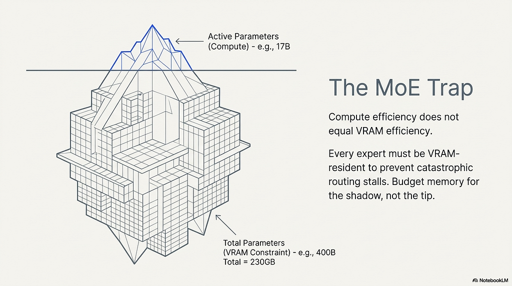
5.3 The MoE VRAM Trap

Mixture-of-Experts [MoE] architectures introduce a VRAM accounting problem that catches even experienced engineers. The trap is simple to describe and surprisingly common to fall into.

An MoE model activates only a subset of its “expert” sub-networks for any given token. A model with 120B total parameters but only 5B active parameters per token uses roughly the same compute per forward pass as a dense 5B model. This makes MoE architectures efficient in FLOPs per token. It does not make them efficient in memory.

Every expert must be resident in VRAM regardless of whether it is active on the current token. The routing mechanism that selects which experts to activate must be able to dispatch to any of them instantly. If an expert is not in VRAM when selected, the forward pass stalls waiting for it to be loaded, which destroys latency. The consequence is that the active parameter count is irrelevant for VRAM budgeting. The total parameter count is what determines memory consumption.

The numbers make this concrete. Mixtral 8x7B has 13B active parameters but 47B total, requiring approximately 28GB at 4-bit. DeepSeek-V2 has 21B active but 236B total, consuming roughly 140GB. Llama-4 Scout has 17B active but 400B total, demanding approximately 230GB at 4-bit. An engineer who budgets VRAM based on the active parameter count will underestimate memory requirements by a factor of 3x to 23x depending on the architecture.

MoE models are also more sensitive to aggressive quantization than their dense counterparts. In a dense model, weight redundancy provides a buffer that absorbs quantization error. In an MoE model, each expert is a smaller, more specialized sub-network with less internal redundancy. Quantizing too aggressively can cause the router to misallocate tokens to the wrong experts, a failure mode unique to MoE architectures. The general recommendation is to avoid Q4_K_M for MoE models and prefer Q5_K_M or higher to keep the routing mechanism stable.

Chapter 6: The Quantization Floor and QAT

When Compression Hits a Wall, and How to Train Through It

The VRAM constraints from Chapter 5 push toward lower bit-widths. But there is a floor below which compression destroys more than it saves, and that floor depends on model size.

6.1 Model Size Determines the Safe Floor

The relationship between model size and quantization tolerance is not linear. It is a cliff.

A 70B parameter model quantized to 4-bit can retain nearly all of its FP16 performance. The weight space is so large and so redundant that rounding millions of weights to their nearest 4-bit representation still leaves enough intact signal for the model to function near its original quality. The redundancy absorbs the error. As model size decreases, the tolerance shrinks rapidly. A 7B model at the same 4-bit precision shows noticeable degradation that may or may not be acceptable depending on the task. A sub-3B model at 4-bit can lose enough fidelity that reasoning, instruction-following, and coherent generation visibly collapse. The weight space is simply too small. There is not enough redundancy to absorb quantization error at that compression level, and every rounding decision affects a proportionally larger share of the model’s total capacity.

The exact retention percentages depend on the specific model, architecture, benchmark, and quantization method. But the general pattern holds across the community’s experience with deploying quantized models. For models above 70B parameters, 4-bit quantization is generally safe. For 14B to 30B models, 5-bit quantization provides a better quality-to-size trade-off. For 7B to 8B models, 6-bit quantization should be the default unless domain-specific evaluation explicitly confirms that a lower bit-depth preserves task performance. For models below 3B parameters, 8-bit quantization is the conservative starting point, and even that may require validation.

The practical implication for anyone deploying a small, specialized model, a fine-tuned 1.5B or 3B model trained for a narrow task, is that the standard 4-bit deployment path does not apply. The model’s utility depends on precision at a level that 4-bit quantization destroys. Professional deployments of sub-8B models should default to 6-bit or 8-bit quantization and only drop lower after extensive task-specific evaluation confirms the degradation is acceptable.

6.2 Quantization-Aware Training as Recovery

Post-training quantization, whether GPTQ, AWQ, or GGUF K-quants, treats quantization as something that happens to a finished model. The model is trained at full precision, then compressed afterward. The model never “sees” the quantization error during training and has no opportunity to adapt to it.

Quantization-Aware Training [QAT] inverts this relationship. Instead of compressing a model that was trained at full precision, QAT simulates the target quantization during the training process itself. The model learns to produce correct outputs despite operating at reduced precision.

The mechanism works through “fake quantization” modules inserted into the model’s linear layers using the torchao integration within Unsloth. During the forward pass, weights and activations are rounded to their target lower-precision representation, exactly as they would be in the final quantized model. The model computes its output using these degraded values. During the backward pass, gradients flow at full precision, updating the weights normally. The model experiences the quantization error at every training step and learns to compensate for it, adjusting its weight distribution so that the rounded values still produce correct outputs.

QAT can recover a significant portion of the accuracy lost to naive post-training quantization. Unsloth’s documentation reports recovery of up to 70% of lost accuracy, with specific results including 66.9% recovery on Gemma3–4B GPQA and 45.5% on Gemma3–12B BBH. Separately, the PyTorch TorchAO team has reported up to 71.6% recovery with NVFP4 QAT in Axolotl workflows. Exact recovery varies by model and benchmark, but the direction is consistent. For sub-4-bit targets, 2-bit or 3-bit precisions needed for edge deployment or mobile inference, this recovery is often the difference between a usable model and one that produces nonsense. Standard post-training quantization at 2-bit or 3-bit is almost always insufficient. QAT is not optional at those compression levels. It is the mechanism that makes them viable at all.

The critical operational requirement is that the fine-tuning and quantization stages must be planned together. A model cannot be QAT-trained after the fact. The fake quantization modules must be present during training, and the target bit-depth must be known before training begins. The model is trained specifically for its deployment precision. A model QAT-trained for 4-bit deployment is not optimized for 2-bit, and vice versa. This couples the training decision to the deployment decision in a way that post-training quantization explicitly avoids.

For the sub-3B models from Section 6.1 where post-training quantization at 4-bit already causes unacceptable degradation, QAT at 4-bit can recover much of the lost quality. For any model where the deployment target is below 4 bits, QAT is the only reliable path. The trade-off is workflow complexity. QAT requires knowing the deployment precision before training starts, allocating training compute for the quantization-aware fine-tuning pass, and accepting that the resulting model is optimized for one specific bit-depth.

Chapter 7: Deployment Routing and Operational Survival

The Final Decision Layer

Every preceding chapter built a piece of the post-training pipeline. This chapter assembles those pieces into a routing decision and covers the operational failure modes that live outside the math entirely.

7.1 The Deployment Decision Matrix

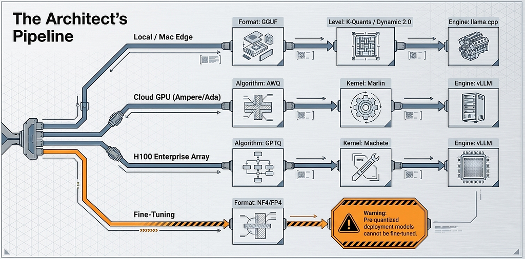
The deployment target determines the format, and the format determines which optimizations from the previous chapters apply. Four deployment surfaces cover virtually all production scenarios, and each one maps to a specific stack.

CPU, local machines, and Mac. The GGUF format running through llama.cpp or Ollama is the primary choice. This stack prioritizes quality and cross-platform compatibility over raw throughput. K-quants and Dynamic 2.0 from Chapter 3 apply here. The quantization level is chosen based on the VRAM or unified memory budget from Chapter 5.

GPU cloud serving with NVIDIA hardware. AWQ or GPTQ from Chapter 2 paired with the Marlin kernel from Chapter 4, served through vLLM or TGI. This stack is designed for throughput, processing multiple concurrent requests in parallel. The Marlin kernel is what converts quantization compression into actual token-per-second gains at batch sizes up to 16 or 32.

H100 enterprise clusters. GPTQ paired with the Machete kernel from Chapter 4. This stack targets high-concurrency enterprise API serving at batch sizes of 64 to 256 where Machete’s Hopper-native optimizations deliver the highest throughput.

Training. Only the bitsandbytes NF4/FP4 format supports fine-tuning with LoRA. This is a hard boundary. A pre-quantized GGUF file cannot be fine-tuned. A GPTQ model cannot be fine-tuned. A practitioner who receives a quantized model and needs to adapt it must either obtain the original FP16 weights or retrain from a base model. The quantization formats covered in this episode are deployment formats, not training formats. Episode 1 covered the bitsandbytes NF4 precision stack used during training, and that remains the only viable path for parameter-efficient fine-tuning on quantized base weights.

7.2 The Chat Template and EOS Trap

The most common post-export failure mode has nothing to do with quantization quality, kernel selection, or VRAM. It is a metadata problem.

A model fine-tuned with Llama-3-Instruct formatting expects a specific sequence of special tokens to delimit user input from assistant responses. A model trained with ChatML expects a different set of tokens. When the inference engine applies the wrong template, the model cannot identify where the user’s message ends and where its own generation should begin. The output is not subtly degraded. It is gibberish. Incoherent token sequences that look like a corrupted model but are actually a perfectly functional model receiving malformed input.

The EOS [End of Sequence] token compounds this problem. If the inference engine does not correctly recognize the model’s EOS token, generation never terminates. The model produces its response, reaches the point where it would normally stop, and continues generating. The result is infinite repetition, hallucinated continuations, or degraded text that loops on itself.

Unsloth mitigates part of this by embedding template metadata directly into GGUF files. But different inference engines, Ollama, llama.cpp, and vLLM, may interpret that embedded metadata differently. The safe practice is to never rely on auto-detection. Force the chat template explicitly in the inference engine’s configuration. Verify that the EOS token matches what was used during training.

7.3 The Complete Pipeline

The full post-training pipeline, assembled from every chapter in this episode, follows a strict sequence where each step depends on the integrity of the one before it.

Merge to FP16 first. This is the canonical source of truth from Chapter 1. Verify the merge is clean, that no recursive merging occurred, and store this checkpoint before doing anything else.

Select the quantization format based on the deployment target from the matrix above. If targeting local deployment, export to GGUF using the appropriate K-quant or Dynamic 2.0 level from Chapter 3. If targeting GPU cloud serving, quantize with AWQ or GPTQ from Chapter 2 and pair with the correct kernel from Chapter 4. If the model is sub-8B, apply the quantization floor guidance from Chapter 6 and consider QAT if the target precision is sub-4-bit.

Calculate the VRAM budget from Chapter 5 before committing to a quantization level. The model weights, the KV cache at the target context length, and the activation memory must all fit within the available hardware. For MoE architectures, budget based on total parameters, not active parameters.

Evaluate the quantized model on task-specific data. Standard perplexity benchmarks on generic datasets will not reveal calibration overfitting in GPTQ, will not catch template mismatches, and will not expose the degradation patterns that appear in sub-8B models at aggressive bit-depths. The evaluation must use data from the actual deployment distribution, testing the actual outputs the model will produce in production.

This episode covered the entire lifecycle after training ends. The merged checkpoint. The compression algorithms. The format ecosystem. The hardware kernels. The memory constraints. The model-size boundaries. The operational traps. Each one is a decision point with specific failure modes, and each one interacts with decisions made at the other points. The model that emerges from this pipeline is not the same model that finished training. It is a compressed, formatted, hardware-targeted derivative of the FP16 original. Every transformation in that pipeline is now visible, so that when something goes wrong in production, the search space for the cause is a structured map rather than a black box.

Connect with me: https://www.linkedin.com/in/suchitra-idumina/

LLM Quantization, Kernels, and Deployment: How to Fine-Tune Correctly, Part 5 was originally published in Towards AI on Medium, where people are continuing the conversation by highlighting and responding to this story.

Like 0

Liked Liked