Vector Search on the Edge: Sensor Retrieval with Qdrant Edge on Ubuntu

Most IoT tutorials stop at collection and dashboards. We’re going deeper into the world of local, offline, and sub-millisecond pattern retrieval.

If you’ve ever built a sensor pipeline before, you know how it usually ends. Data flows in, you set some thresholds, draw a pretty chart, and call it a day. And honestly? That’s fine. Until it isn’t.

Thresholds catch obvious failures. Dashboards show you history. But neither of them answers the question that actually matters in production:

“Have I seen this pattern before?”

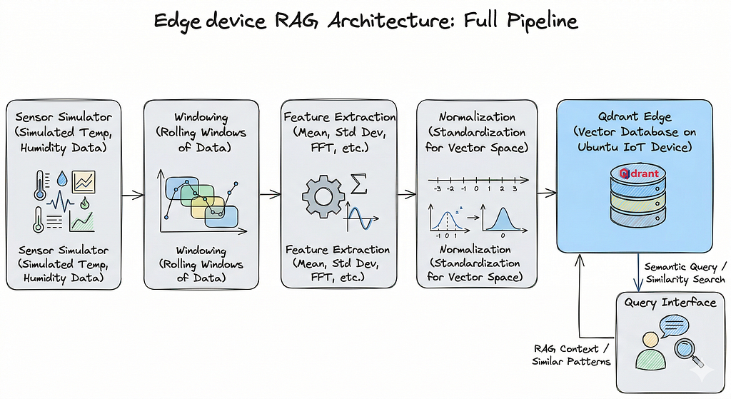
That’s exactly what this article is about: building a local, retrieval-first sensor search system using Qdrant Edge, running entirely on an Ubuntu edge device. No cloud dependency. No heavy model. No physical sensor hardware required; we’ll simulate everything in Python so you can prototype, break things, and iterate fast before touching real devices.

By the end of this article, you’ll have a working system that:

1. Generates realistic multi-sensor data streams
2. Converts time-series windows into searchable vectors
3. Stores them locally with metadata in Qdrant Edge
4. Runs similarity queries with filters to retrieve matching patterns from history

Why Prototype Sensor Search Locally First?

In the world of Edge AI, the “hardware tax” is real. Starting with physical sensors often means spending weeks fighting wiring issues, power fluctuations, and unstable drivers before you even write a single line of retrieval logic. By shifting to a simulation-first workflow on a robust Ubuntu substrate, you move the focus from “plumbing” to architecture.

Prototyping in a local Ubuntu VM serves as the ultimate development sandbox for several mission-critical reasons:

• Eliminating Hardware Friction: You remove the initial barriers to entry by delaying physical setup, allowing for rapid iteration on the actual problem-solving code rather than hardware troubleshooting.
• High-Velocity Debugging: Local environments allow for instantaneous restarts and real-time log monitoring without the latency or “wear and tear” of physical device cycling.
• Absolute Reproducibility: Because the environment is containerized or VM-based, the stack remains consistent across your entire team. Furthermore, the Qdrant Edge storage files are fully portable once you’ve built your vector database locally, you can simply move the file to your target hardware, and it will function identically.
• A Proof of Concept: It provides a clean, noise-free space to validate your retrieval patterns and tune your feature pipeline. This creates a vital separation of concerns: you prove “Does the search work?” independently of “Does the sensor work?”.
• Streamlined Onboarding: New developers can jump into the project and start contributing to the AI logic immediately, without needing a physical kit mailed to them.

The central challenge in sensor workflows is that historical data, while collected in logs and dashboards, is not searchable in any meaningful way. The core idea of this retrieval-first tutorial is that search is the missing layer in many sensor workflows.

Note: After successful installation of Ubuntu in your VirtualBox, don’t forget to run the following commands:

sudo apt update && sudo apt upgrade -y 
sudo apt install python3-pip python3-venv -y

This will install and update all the required dependencies.

The Problem with Standard Sensor Monitoring

The current approach to sensor monitoring has significant drawbacks:

• Simple threshold alerts, like if temperature > 80: alert(), are reactive and often trigger too late.
• Dashboards, while visually appealing, are passive and require manual effort to spot anomalies.
• Raw logs are cumbersome — they are noisy, lack easy comparison, and are effectively impossible to search in a meaningful way.

What you actually want is something closer to how image search works. You take a new reading, and ask: “Show me the 10 most similar windows from the last 30 days, but only from Sensor B in Zone C.”

That’s vector search with metadata filtering. And it’s genuinely useful.

The ability to effectively search and analyze sensor logs is crucial for various applications. For instance, being able to spot pre-failure vibration signatures can prevent catastrophic motor failure, allowing for timely maintenance. Also, correlating anomalies, such as unexpected humidity readings across different zones, can reveal underlying environmental issues or system interactions. A well-indexed log system also facilitates the retrieval of historical patterns, such as finding past temperature readings that closely resemble the current data, which is vital for predictive modeling and understanding long-term trends. Finally, the capacity to filter anomaly-like windows by specific sensor types and precise time ranges ensures that investigations are focused and efficient, leading to faster root cause analysis.

Thresholds only catch what you already knew you had to to look for. Dashboards show you history without letting you query it. What’s missing is the ability to search sensor behavior the way you’d search a knowledge base.

This is where vector search enters. By converting short windows of sensor readings into feature vectors, you can use cosine similarity to retrieve the most similar historical patterns with metadata filters on top to narrow by sensor type, location, time bucket, or anomaly class.

Why Use Qdrant Edge?

There are a few practical reasons this setup uses Qdrant Edge specifically.

It runs entirely locally with no external service, no API key, no network required. On edge hardware with limited connectivity — that matters a lot. The footprint is small, the setup is simple, and it handles both vector search and metadata filtering in a single query. You don’t need a separate database for the payload filtering — it’s all in one place.

Qdrant Edge uses a shard-based local storage model. You create a shard directory, configure your vector size and distance metric, and it handles the rest. The storage file for the Qdrant vector database, created on the edge device, is notably powerful and portable. This allows for simple transfer to any other device; running the test code will work identically, eliminating the need to regenerate the vector database.

Setting Up the Environment

Ubuntu is a robust, enterprise-grade operating system that provides a stable and secure substrate for complex edge AI deployments. It offers native, highly optimized support for modern AI frameworks and Python environments (latest Python Version), making it a superior choice for running continuous vector databases like Qdrant.

To set up your Ubuntu environment for this RAG edge project, you need to create a reproducible sandbox that mimics a production IoT deployment. This involves initializing a Python virtual environment to isolate dependencies and installing a specific stack of scientific and vector-search libraries.

To begin, create a virtual environment and then install the necessary libraries using the commands provided below.

# Create the environment
python3 -m venv qdrant_env

# Activate the environment
source qdrant_env/bin/activate

pip install numpy pandas matplotlib seaborn qdrant-edge-py scipy scikit-learn

Imports you’ll need in your script:

import numpy as np
import pandas as pd
import matplotlib.pyplot as plt
import seaborn as sns
from scipy.stats import skew, kurtosis
from sklearn.preprocessing import StandardScaler
from pathlib import Path
from qdrant_edge import *
import random

Step 1: Simulating Sensor Data

We’d have a fleet of industrial motors and high-fidelity sensors wired up to our Ubuntu nodes. In the real world of rapid prototyping, hardware is friction. To bypass this, we build a SensorSimulator — a Python class designed not just to generate numbers, but to mimic the “behavioral signatures” of physical assets.

• The Baseline: The rhythmic baseline of a machine (sine waves).
• The Noise: The inevitable entropy of any physical system (Gaussian distribution).
• The Anomalies: The sudden spikes or sustained deviations like Bearing Wear.

class SensorSimulator:
    def __init__(
        self,
        duration_minutes: int = 60, # Total simulation time in minutes
        sampling_rate_hz: int = 1, # Data points per second
        amplitude: float = 10.0, # Base amplitude of the signal
        frequency: float = 0.01, # Frequency of baseline periodic behavior
        noise_level: float = 0.5, # Magnitude of random noise
        spike_magnitude: float = 5.0, # Magnitude of sudden spikes
        spike_frequency_minutes: int = 10, # How often spikes occur in minutes
        anomaly_magnitude: float = 15.0, # Magnitude of repeated anomaly signatures
        anomaly_duration_seconds: int = 30, # Duration of each anomaly in seconds
        anomaly_frequency_minutes: int = 17, # How often anomalies occur in minutes
        random_seed: int = 42, # Seed for reproducibility
        start_datetime_str: str = None # Custom start datetime string
    ):
        self.duration_minutes = duration_minutes
        self.sampling_rate_hz = sampling_rate_hz
        self.amplitude = amplitude
        self.frequency = frequency
        self.noise_level = noise_level
        self.spike_magnitude = spike_magnitude
        self.spike_frequency_minutes = spike_frequency_minutes
        self.anomaly_magnitude = anomaly_magnitude
        self.anomaly_duration_seconds = anomaly_duration_seconds
        self.anomaly_frequency_minutes = anomaly_frequency_minutes
        self.random_seed = random_seed
        self.start_datetime_str = start_datetime_str

        np.random.seed(self.random_seed)

        self.total_samples = self.duration_minutes * 60 * self.sampling_rate_hz
        self.time = np.arange(self.total_samples) / self.sampling_rate_hz

    def _add_baseline(self, offset: float = 0):
        # Simulates a periodic baseline behavior (e.g., daily cycle)
        return self.amplitude * np.sin(2 * np.pi * self.frequency * self.time / 60) + offset

    def _add_noise(self):
        # Adds random fluctuations to the data
        return np.random.normal(0, self.noise_level, self.total_samples)

    def _add_spikes(self):
        # Adds sudden, short-lived increases or decreases
        spikes = np.zeros(self.total_samples)
        spike_interval_samples = self.spike_frequency_minutes * 60 * self.sampling_rate_hz
        if spike_interval_samples > 0:
            num_spikes = self.total_samples // spike_interval_samples
            for i in range(1, num_spikes + 1):
                spike_idx = i * spike_interval_samples + np.random.randint(-self.sampling_rate_hz * 5, self.sampling_rate_hz * 5)
                if 0 <= spike_idx < self.total_samples:
                    spikes[spike_idx] += self.spike_magnitude * np.random.choice([-1, 1])
        return spikes

    def _add_anomalies(self):
        anomalies = np.zeros(self.total_samples)
        anomaly_interval_samples = self.anomaly_frequency_minutes * 60 * self.sampling_rate_hz
        anomaly_duration_samples = self.anomaly_duration_seconds * self.sampling_rate_hz

        if anomaly_interval_samples > 0 and anomaly_duration_samples > 0:
            num_anomalies = self.total_samples // anomaly_interval_samples
            for i in range(1, num_anomalies + 1):
                start_idx = i * anomaly_interval_samples
                end_idx = min(start_idx + anomaly_duration_samples, self.total_samples)
                if start_idx < self.total_samples:
                    anomalies[start_idx:end_idx] += self.anomaly_magnitude * np.random.choice([-1, 1])
        return anomalies

    def generate_data(self, sensor_type: str = 'Temperature') -> pd.DataFrame:
        # Generate individual components
        baseline_offset = {'Temperature': 20, 'Humidity': 60, 'Vibration': 0, 'Air-quality': 50}.get(sensor_type, 0)
        baseline = self._add_baseline(offset=baseline_offset)
        noise = self._add_noise()
        spikes = self._add_spikes()
        anomalies = self._add_anomalies()

        simulated_data = baseline + noise + spikes + anomalies

        if self.start_datetime_str:
            start_timestamp = pd.to_datetime(self.start_datetime_str)
            time_deltas = pd.to_timedelta(self.time, unit='s')
            timestamps = start_timestamp + time_deltas
        else:
            timestamps = pd.to_datetime(self.time, unit='s')

        df = pd.DataFrame({
            'timestamp': timestamps,
            'sensor_type': sensor_type,
            'value': simulated_data
        })
        return df

print("SensorSimulator class defined successfully.n")




Generating the Sensor Data:

simulator = SensorSimulator(duration_minutes=7200, sampling_rate_hz=1, start_datetime_str='2026-03-01 00:00:00')

sensor_types = ['Temperature', 'Humidity', 'Vibration', 'Air-quality']
all_sensor_data = []

for sensor_type in sensor_types:
    df_sensor = simulator.generate_data(sensor_type)
    all_sensor_data.append(df_sensor)

df_all_sensors = pd.concat(all_sensor_data, ignore_index=True)


print(df_all_sensors.head(), "n")
print(f"Shape of the combined DataFrame: {df_all_sensors.shape}n")
# Shape of combined DataFrame: (1728000, 3)

5 days × 4 sensor types × 1 reading/second = 1.7 million data points. That’s a realistic volume for an edge device to handle over a short deployment window.

This graph illustrates a representative sample of simulated sensor data collected over a 600-minute period.

Step 2: Windowing the Data

Raw sensor data is just a stream of numbers, a “point-in-time” snapshot that, in isolation, tells us very little. If a temperature sensor reads 35°C, is that a normal operating peak or the start of a catastrophic bearing failure? You can’t tell by looking at a single dot; you need to see the shape of the signal over time.

To make this searchable, we use a technique called windowing. Instead of treating every individual second as a data point, we group our readings into meaningful temporal blocks. Think of it like taking a long video and cutting it into short, 1-minute clips. Each “clip” or window now contains the narrative of what happened in that sixty-second interval.

The Strategy: From Streams to Snapshots

In our Ubuntu-based RAG architecture, we process these windows locally. We iterate through each unique sensor Temperature, Humidity, Vibration, Air-Quality and “resample” the timeline into 1-minute buckets. This creates a structured history where every row in our final dataframe represents a “behavioral window” rather than a lone measurement.

window_size = '1min'
df_all_sensors['timestamp'] = pd.to_datetime(df_all_sensors['timestamp'])
windowed_data = []

for sensor_type in df_all_sensors['sensor_type'].unique():
    df_sensor_type = df_all_sensors[df_all_sensors['sensor_type'] == sensor_type].set_index('timestamp')
    df_window = df_sensor_type['value'].resample(window_size).apply(list).reset_index()
    df_window['sensor_type'] = sensor_type
    df_window.rename(columns={'value': 'window_values'}, inplace=True)
    windowed_data.append(df_window)

df_windowed = pd.concat(windowed_data, ignore_index=True)

print(f"Windowed data created successfully with a window size of {window_size}. First 5 rows:n")
print(df_windowed.head(), "n")
print(f"Shape of the windowed DataFrame: {df_windowed.shape}n")
# Shape: (28800, 3) — 7200 minutes × 4 sensor types

Each row now holds a list of 60 readings, one minute of sensor behavior ready to be turned into a feature vector.

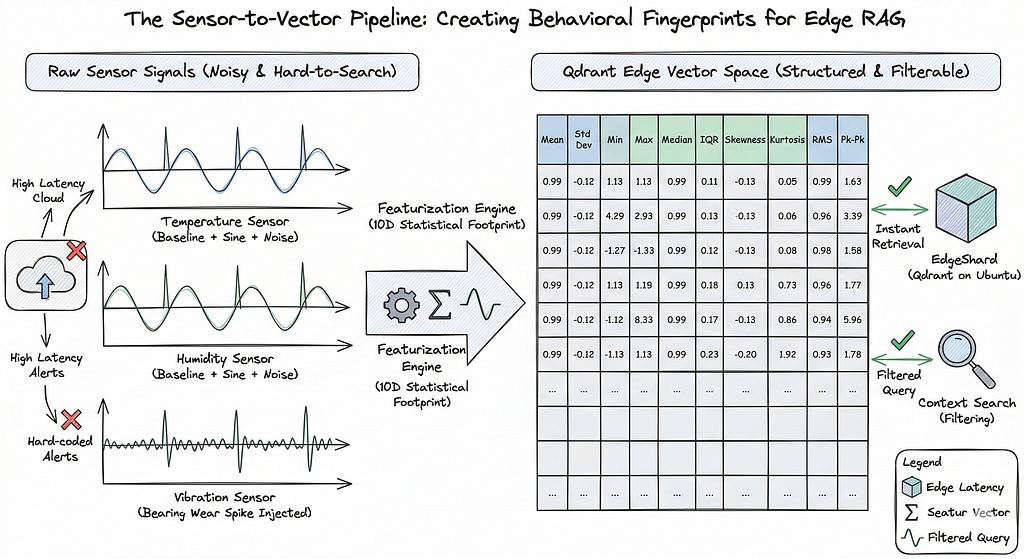
Step 3: Feature Extraction

This is where things get interesting. We don’t need a neural network to turn these windows into meaningful vectors. Ten statistical features capture the shape, spread, and dynamics of each window well enough for pattern retrieval.

def extract_features(window_values, sampling_rate_hz=1):
    if not window_values:
        return pd.Series({
            'mean_value': np.nan,
            'std_dev': np.nan,
            'min_value': np.nan,
            'max_value': np.nan,
            'median_value': np.nan,
            'iqr_value': np.nan,
            'skewness': np.nan,
            'kurtosis': np.nan,
            'rms_value': np.nan,
            'peak_to_peak': np.nan,
        })

    values_arr = np.array(window_values)
    num_samples = len(values_arr)

    q1 = np.percentile(values_arr, 25)
    q3 = np.percentile(values_arr, 75)

    # Basic statistical features
    mean_val = np.mean(values_arr)
    std_dev_val = np.std(values_arr)
    min_val = np.min(values_arr)
    max_val = np.max(values_arr)
    median_val = np.median(values_arr)
    iqr_val = q3 - q1
    skewness_val = skew(values_arr)
    kurtosis_val = kurtosis(values_arr)
    rms_val = np.sqrt(np.mean(np.square(values_arr)))
    peak_to_peak_val = max_val - min_val


    return pd.Series({
        'mean_value': mean_val,
        'std_dev': std_dev_val,
        'min_value': min_val,
        'max_value': max_val,
        'median_value': median_val,
        'iqr_value': iqr_val,
        'skewness': skewness_val,
        'kurtosis': kurtosis_val,
        'rms_value': rms_val,
        'peak_to_peak': peak_to_peak_val,
    })

df_features = df_windowed['window_values'].apply(lambda x: extract_features(x, sampling_rate_hz=1))

columns_to_drop = [
    'mean_value', 'std_dev', 'min_value', 'max_value', 'median_value',
    'iqr_value', 'skewness', 'kurtosis', 'feature_vector', 'rms_value', 'peak_to_peak'
]

df_windowed = df_windowed.drop(columns=columns_to_drop, errors='ignore')
df_windowed = pd.concat([df_windowed, df_features], axis=1)

print("Features extracted and added to df_windowed. First 5 rows with new features:n")
print(df_windowed.head(), "n")
print(f"Shape of the DataFrame with features: {df_windowed.shape}n")

To build a robust retrieval system, we extract features that describe the signal’s central tendency, its spread, and its shape:

• Mean & Median: These establish the baseline operating level. A sudden shift in the mean often signals a change in the environment or a steady “drift” in the asset’s health.
• Standard Deviation (Std Dev) & RMS: These measure the “energy” and intensity of the signal. In vibration sensors, a higher RMS (Root Mean Square) is a classic indicator of increased mechanical stress.
• Min/Max & Peak-to-Peak: These capture the extremes. The Peak-to-Peak value is vital for catching sudden, violent shocks that might be averaged out in other calculations.
• IQR (Interquartile Range): Unlike standard deviation, IQR is robust against outliers, helping us understand the “normal” spread of the data within that minute.
• Skewness: This measures the symmetry of the signal. If a sensor starts reporting more “high” spikes than “low” ones, the skewness will shift, indicating an unbalanced state.
• Kurtosis: Perhaps the most important for anomaly detection. It measures the “tailedness” or “peakedness” of the data. High kurtosis means the signal is producing frequent, extreme outliers, the “sharp” spikes typical of bearing cracks.

Step 4: Normalization and Vector Representation

The features are on different scales meaning temperature is ~20, while kurtosis might be near zero. Before storing them as vectors, we normalize using StandardScaler so no single feature dominates the similarity calculation.

feature_columns = [
    'mean_value', 'std_dev', 'min_value', 'max_value', 'median_value',
    'iqr_value', 'skewness', 'kurtosis', 'rms_value', 'peak_to_peak'
]

scaler = StandardScaler()
df_windowed[feature_columns] = scaler.fit_transform(df_windowed[feature_columns])
df_windowed['feature_vector'] = df_windowed[feature_columns].values.tolist()

Each row in df_windowed now has a feature_vector, a 10-dimensional normalized representation of 60 seconds of sensor behavior. That’s what goes into Qdrant.

It is a common misconception that vector search is strictly reserved for high-dimensional text embeddings or massive Transformer models. In this edge-focused architecture, we prove that vectors do not need to originate from a large ML model to be powerful. By using lightweight numeric features, statistical signatures of our sensor windows, we can capture the “essence” of a signal without the computational overhead of deep learning. This demonstrates that vector search is a versatile retrieval pattern for any structured data, allowing us to find complex sensor behaviors like “Bearing Wear” through simple, efficient mathematical footprints.

Step 5: Setting up Qdrant Edge

With our features extracted and normalized, we move into the core components of the architecture: the Retrieval Engine. In a traditional cloud-based RAG setup, you would connect to a remote cluster via an API. However, for an edge deployment on Ubuntu, we need something that lives inside the process minimizing latency and ensuring 100% offline capability.

This is where Qdrant Edge comes in. It isn’t just a database; it’s a lightweight, high-performance vector shard that runs directly on your local storage.

SHARD_DIRECTORY = "./qdrant-edge-1"
Path(SHARD_DIRECTORY).mkdir(parents=True, exist_ok=True)

VECTOR_DIMENSION = len(df_windowed['feature_vector'].iloc[0])
config = EdgeConfig(
    vectors=EdgeVectorParams(size=VECTOR_DIMENSION, distance=Distance.Cosine),
    )
edge_shard = EdgeShard.create(SHARD_DIRECTORY, config)

Reference: qdrant_documentation

Cosine distance makes sense here. We care about the shape and direction of the feature vector, not its magnitude. Two windows with the same pattern but different absolute values should still be considered similar.

Step 6: Storing Vectors with Metadata

Storing a vector by itself is like having a fingerprint without a name attached to it. In an industrial edge environment, the “where” and “when” are just as critical as the “what.” To make our RAG system truly operational, we need to wrap our 10-dimensional feature vectors in Metadata (also known as a “payload” in Qdrant).

This metadata transforms a raw mathematical footprint into a searchable historical record. By adding fields like sensor_type, location, and anomaly_label, we enable the system to perform complex, filtered queries such as searching for “vibration spikes” specifically in “Zone_B.”

points = []

sensor_clocks = {s: 0 for s in df_windowed['sensor_type'].unique()}
for index, row in df_windowed.iterrows():
    s_type = row['sensor_type']
    local_minute = sensor_clocks[s_type]

    if local_minute > 0 and local_minute % 17 == 0:
        label = 'Bearing Wear'
    elif local_minute > 0 and local_minute % 10 == 0:
        label = 'Sudden Spike'
    else:
        label = 'Normal'

    sensor_clocks[s_type] += 1

    metadata = {
        'sensor_type': row['sensor_type'],
        'timestamp': row['timestamp'].isoformat(),
        'source_id': random.randint(100, 999),
        'location': random.choice(['Zone_A', 'Zone_B', 'Zone_C', 'Zone_D']),
        'simulation_mode': row.get('simulation_mode', 'standard'),
        'anomaly_label': label
    }

    point = Point(
        id=index,
        vector=row['feature_vector'],
        payload=metadata
    )
    points.append(point)

print(f"Successfully created {len(points)} Point objects.n")
print("Sample metadata from the first point:n")
print(points[73].payload, "n")

edge_shard.update(
    UpdateOperation.upsert_points(
        points
    )
)

print(f"Successfully upserted {len(points)} enriched points to collection '{SHARD_DIRECTORY}'.n")

count = edge_shard.count(CountRequest(exact=True))
print(f"Total points count: {count}n")
edge_shard.update(
    UpdateOperation.create_field_index("timestamp", PayloadSchemaType.Datetime)
)

Each Point in our Qdrant Edge shard carries the following identity:

• sensor_type: This identifies the data source (Temperature, Humidity, etc.). In our simulation, it allows us to prove that we can isolate search results to a specific signal type.
• timestamp: A high-resolution ISO-8601 string. Since our data is synthetic, this lets us “travel back in time” to test if we can retrieve patterns from specific historical windows.
• source_id: A randomized three-digit identifier (100–999).
• location: Randomly assigned to ‘Zone_A’ through ‘Zone_D’. This is crucial for verifying Spatial Filtering, ensuring we only find anomalies relevant to a specific part of the factory floor.
• anomaly_label: Our “Gold Standard” label (Normal, Sudden Spike, or Bearing Wear). We use this to verify the accuracy of our search; if we query a “Bearing Wear” signal and Qdrant returns points with this label, our system is proven.

We also create a datetime index on the timestamp field so range queries run efficiently:

edge_shard.update(
    UpdateOperation.create_field_index("timestamp", PayloadSchemaType.Datetime)
)

In many RAG tutorials, the story ends once you find the “nearest neighbor” in a vector space. But in a real-world industrial environment, especially when running on an Ubuntu edge node, similarity alone is often a blunt instrument. If your vibration sensor detects a suspicious harmonic, simply finding “something similar” in your history isn’t enough. You need to find something similar that actually matters in the current context.

The Limitation of Pure Similarity

Imagine a factory with fifty different motors. If Motor #5 starts showing signs of bearing wear, a pure similarity search might return a “match” from Motor #12 because their vibration signatures look mathematically alike. However, Motor #12 is a different model, operates under a different load, and is located in a different climate zone. That “similar” result is functionally useless -> it’s noise.

Retrieval with Constraints: Real-World Scenarios

In an edge context, retrieval must be governed by operational constraints. This is why we spent time enriching our points with a detailed payload. Consider these mission-critical queries that pure vector search would fail, but filtered RAG solves:

• Machine-Specific Diagnostics: “Find vibration patterns similar to this one, but only from this specific source_id”.
• Temporal Relevance: “Search for similar spikes, but only within the last 7 days of historical logs”.
• Environmental Context: “Find similar anomalies, but restrict the search to sensor_type: humidity data”.
• Scenario Validation: “Retrieve matching patterns, but only from the simulation_mode: standard dataset to avoid test-run contamination”.

By combining vector similarity with high-performance Boolean filters, Qdrant allows us to narrow down the search space before or during the similarity calculation. On a resource-constrained Ubuntu device, this isn’t just a feature; it’s an optimization.

Step 7: Querying the System

Now comes the part that makes this actually useful.

For vector search to be accurate, the “query vector” (the live data) and the “base vectors” (the historical data) must exist in the same mathematical space. This function ensures perfect symmetry by calculating the exact same statistical parameters we used during the ingestion phase.

def features(live_window_raw):
    print("Raw live window data:n", live_window_raw, "n")

    return np.array([
    np.mean(live_window_raw),
    np.std(live_window_raw),
    live_window_raw.min(),
    live_window_raw.max(),
    np.median(live_window_raw),
    np.percentile(live_window_raw, 75) - np.percentile(live_window_raw, 25),
    skew(live_window_raw),
    kurtosis(live_window_raw),
    np.sqrt(np.mean(np.square(live_window_raw))),
    live_window_raw.max() - live_window_raw.min()

]).reshape(1, -1)

We made a helper function which generates the output in a structured way and stores it into a file, output.txt.

def save_search_results(filename, test_name, live_window_raw, live_features, query_vector, results):
    """Save search results to file and print to console"""

    feature_names = ['mean_value', 'std_dev', 'min_value', 'max_value', 'median_value', 'iqr_value', 'skewness', 'kurtosis', 'rms_value', 'peak_to_peak']

    # Prepare output text
    output_lines = []
    output_lines.append("=" * 80)
    output_lines.append(f"TEST: {test_name}")
    output_lines.append("=" * 80)
    output_lines.append("")

    # Raw window data
    output_lines.append("RAW LIVE WINDOW DATA:")
    output_lines.append(str(live_window_raw))
    output_lines.append("")

    # Features extracted
    output_lines.append("EXTRACTED FEATURES:")
    for i, name in enumerate(feature_names):
        output_lines.append(f"  {name}: {live_features[0][i]:.6f}")
    output_lines.append("")

    # Query vector (scaled)
    output_lines.append("QUERY VECTOR (Scaled):")
    output_lines.append(str(query_vector))
    output_lines.append("")

    # Search results
    output_lines.append("SEARCH RESULTS (Top 10 Matches):")
    output_lines.append("-" * 80)

    for idx, hit in enumerate(results, 1):
        output_lines.append(f"Result #{idx}:")
        output_lines.append(f"  Similarity Score: {hit.score:.6f}")
        output_lines.append(f"  Identified Pattern: {hit.payload['anomaly_label']}")
        output_lines.append(f"  Historical Match Time: {hit.payload['timestamp']}")
        output_lines.append(f"  Sensor Type: {hit.payload['sensor_type']}")
        if 'location' in hit.payload:
            output_lines.append(f"  Location: {hit.payload['location']}")
        output_lines.append(f"  Vector: {hit.vector}")
        output_lines.append("-" * 80)

    output_lines.append("n")

    # Print to console
    output_text = "n".join(output_lines)
    print(output_text)

    # Append to file
    with open(filename, 'a') as f:
        f.write(output_text)

Query 1 — Bearing Wear Pattern Retrieval

We simulate a new temperature window with an injected anomaly. Values rise sharply in the middle, mimicking a bearing wear signature:

live_window_raw = np.random.normal(20, 0.5 , 60)
live_window_raw[10:35] += 15
live_features = features(live_window_raw)
query_vector = scaler.transform(live_features)[0].tolist()

result = edge_shard.query(
    QueryRequest(
        query=Query.Nearest(query_vector),
        limit=10,
        with_vector=True,
        with_payload=True,
    )
)

save_search_results('search_results.txt', 'Bearing Wear Temperature',
                   live_window_raw, live_features, query_vector, result)

Reference: Qdrant Vector Search Concepts

Results:

================================================================================
TEST: Bearing Wear Temperature
================================================================================

RAW LIVE WINDOW DATA:
[20.09945228 20.1268545  19.6369997  19.46700812 19.89917426 20.24950434
 20.13884831 19.27802916 19.36262239 19.69492818 34.77829627 34.27980205
 35.34124606 34.86546776 35.24656781 35.02625409 35.29354689 34.59112675
 34.67783562 33.93433694 35.19340315 35.51401838 34.68761839 35.50978984
 35.6446397  35.34417304 34.15772488 35.01975444 34.69143604 33.73297004
 34.72530651 35.08773941 36.19497267 34.8836887  34.43481189 19.48492749
 20.31578151 20.40842651 19.47284595 19.86658255 20.40286383 19.47272972
 20.55263637 19.03620611 19.77312456 20.2100657  19.93702582 20.04215261
 21.14995325 20.02225865 20.45911834 20.33632623 19.91925298 20.59692737
 20.37583753 20.96176554 20.18122934 20.26476427 19.57082966 20.43382523]

EXTRACTED FEATURES:
  mean_value: 26.234290
  std_dev: 7.353147
  min_value: 19.036206
  max_value: 36.194973
  median_value: 20.446472
  iqr_value: 14.737604
  skewness: 0.337919
  kurtosis: -1.866678
  rms_value: 27.245307
  peak_to_peak: 17.158767

QUERY VECTOR (Scaled):
[-0.25189095941116163, 3.8934539471549794, -0.46643315783917183, 0.07496247819889704, -0.4840205830768557, 3.9281945989897324, 0.30855239252241967, -0.5856833315462647, -0.309588108475088, 3.7514323562372827]

SEARCH RESULTS (Top 10 Matches):
--------------------------------------------------------------------------------
Result #1:
  Similarity Score: 0.998665
  Identified Pattern: Bearing Wear
  Historical Match Time: 2026-03-03T08:40:00
  Sensor Type: Temperature
  Location: Zone_A
  Vector: [-0.028729060664772987, 0.5792194604873657, -0.06790333986282349, 0.012674110010266304, -0.043212417513132095, 0.5796058773994446, 0.004736441653221846, -0.0893632248044014, -0.036702949553728104, 0.5583389401435852]
--------------------------------------------------------------------------------
Result #2:
  Similarity Score: 0.998402
  Identified Pattern: Bearing Wear
  Historical Match Time: 2026-03-02T21:54:00
  Sensor Type: Temperature
  Location: Zone_D
  Vector: [-0.04377015680074692, 0.586844801902771, -0.08108190447092056, -0.0022375015541911125, -0.044831790030002594, 0.5802040100097656, 0.0022185237612575293, -0.08570118993520737, -0.051696956157684326, 0.5463052988052368]
--------------------------------------------------------------------------------
Result #3:
  Similarity Score: 0.998339
  Identified Pattern: Bearing Wear
  Historical Match Time: 2026-03-03T11:13:00
  Sensor Type: Temperature
  Location: Zone_D
  Vector: [-0.04139602929353714, 0.582907497882843, -0.07956237345933914, -0.000719793199095875, -0.04113340377807617, 0.5848698019981384, 0.0011993867810815573, -0.08673269301652908, -0.04947102442383766, 0.5462952256202698]
--------------------------------------------------------------------------------

………………………………………………………………….  Upto 10 results

Query 2 — Normal Humidity Baseline

"""### Humidity - Air-Quality"""

live_window_raw = np.random.normal(60, 0.5 , 60)
live_features = features(live_window_raw)
query_vector = scaler.transform(live_features)[0].tolist()
result = edge_shard.query(
 QueryRequest(
 query=Query.Nearest(query_vector),
 limit=10,
 with_vector=True,
 with_payload=True,
 )
)
save_search_results('search_results.txt', 'Humidity - Air-Quality',
 live_window_raw, live_features, query_vector, result)

Results:

—------skipped above results —------
SEARCH RESULTS (Top 10 Matches):
--------------------------------------------------------------------------------
Result #1:
  Similarity Score: 0.999973
  Identified Pattern: Normal
  Historical Match Time: 2026-03-01T06:37:00
  Sensor Type: Humidity
  Location: Zone_C
  Vector: [0.4325069189071655, -0.11341110616922379, 0.43912747502326965, 0.4181174039840698, 0.4316273331642151, -0.09894439578056335, -0.008008246310055256, -0.12869641184806824, 0.44577544927597046, -0.14486420154571533]
--------------------------------------------------------------------------------



Result #2:
  Similarity Score: 0.999972
  Identified Pattern: Normal
  Historical Match Time: 2026-03-01T23:41:00
  Sensor Type: Air-quality
  Location: Zone_D
  Vector: [0.43263763189315796, -0.11015856266021729, 0.4383421540260315, 0.4173826277256012, 0.4317515194416046, -0.10076398402452469, -0.00884172972291708, -0.12905770540237427, 0.4473882019519806, -0.14451512694358826]
--------------------------------------------------------------------------------
Result #3:
  Similarity Score: 0.999941
  Identified Pattern: Normal
  Historical Match Time: 2026-03-03T05:52:00
  Sensor Type: Air-quality
  Location: Zone_A
  Vector: [0.4304860830307007, -0.11234068125486374, 0.4418080449104309, 0.42151549458503723, 0.4305127263069153, -0.10105251520872116, 0.0025364619214087725, -0.12924453616142273, 0.4442521631717682, -0.13988648355007172]
--------------------------------------------------------------------------------
Result #4:
  Similarity Score: 0.999931
  Identified Pattern: Normal
  Historical Match Time: 2026-03-05T21:02:00
  Sensor Type: Air-quality
  Location: Zone_D
  Vector: [0.43112680315971375, -0.11147137731313705, 0.43910953402519226, 0.41814643144607544, 0.4327910542488098, -0.10624738782644272, -0.01093031745404005, -0.12489212304353714, 0.44590869545936584, -0.14453844726085663]
--------------------------------------------------------------------------------
Result #5:
  Similarity Score: 0.999926
  Identified Pattern: Normal
  Historical Match Time: 2026-03-05T18:55:00
  Sensor Type: Humidity
  Location: Zone_B
  Vector: [0.4297553598880768, -0.11720667034387589, 0.44098153710365295, 0.4190673828125, 0.4306878447532654, -0.10905366390943527, -0.000717424787580967, -0.12824660539627075, 0.4413827955722809, -0.15112702548503876]
--------------------------------------------------------------------------------

. .. . . . . . . . till 10 results

Notice something important in these results: the top matches include both Humidity and Air-Quality sensors. That makes sense: both signals hover around similar values with similar statistical shapes. Without filtering, Qdrant correctly returns the most similar vectors regardless of sensor type.

Which brings us to the most useful part.

Query 3 — Filter-Based Search (Humidity Only)

Same query vector, but now we constrain results to humidity sensors only:

live_window_raw = np.random.normal(60, 0.5 , 60)
live_features = features(live_window_raw)
query_vector = scaler.transform(live_features)[0].tolist()

search_filter = Filter(
    must=[
        FieldCondition(
            key="sensor_type",
            match=MatchTextAny(text_any="Humidity"),
        ),
    ]
)

result = edge_shard.query(
    QueryRequest(
        query=Query.Nearest(query_vector),
        filter = search_filter,
        limit=10,
        with_vector=True,
        with_payload=True,
    )
)

save_search_results('search_results.txt', 'Filter-based Search (Humidity)',
                   live_window_raw, live_features, query_vector, result)

Results:

***** trimmed some results and values ****
================================================================================
TEST: Filter-based Search (Humidity)
================================================================================


SEARCH RESULTS (Top 10 Matches):
--------------------------------------------------------------------------------
Result #1:
  Similarity Score: 0.999914
  Identified Pattern: Normal
  Historical Match Time: 2026-03-04T08:53:00
  Sensor Type: Humidity
  --------------------------------------------------------------------------------
Result #2:
  Similarity Score: 0.999903
  Identified Pattern: Normal
  Historical Match Time: 2026-03-04T13:47:00
  Sensor Type: Humidity
--------------------------------------------------------------------------------
Result #3:
  Similarity Score: 0.999903
  Identified Pattern: Normal
  Historical Match Time: 2026-03-04T16:19:00
  Sensor Type: Humidity
--------------------------------------------------------------------------------
Result #4:
  Similarity Score: 0.999845
  Identified Pattern: Normal
  Historical Match Time: 2026-03-01T18:15:00
  Sensor Type: Humidity
-------------------------------------------------------------------------------
Result #5:
  Similarity Score: 0.999844
  Identified Pattern: Normal
  Historical Match Time: 2026-03-02T00:55:00
  Sensor Type: Humidity
--------------------------------------------------------------------------------
Result #6:
  Similarity Score: 0.999804
  Identified Pattern: Normal
  Historical Match Time: 2026-03-01T20:49:00
  Sensor Type: Humidity
--------------------------------------------------------------------------------

Query 4 — Advanced Filter: Humidity + Zone_B + DateTime Range

This is where things get genuinely powerful. We inject a humidity anomaly (the += 15 shift) and search for similar patterns — but only from Zone_B, only for humidity sensors, and only within the first 4 hours of March 1st:

#########   Filters   #########
#  Sensor-type = humidity
#  location = Zone_B
#  DateTime in range (00:00:00 to 04:00:00) same date

search_filter = Filter(
    must=[
        FieldCondition(
            key="sensor_type",
            match=MatchTextAny(text_any="Humidity"),
        ),
        FieldCondition(
            key="location",
            match=MatchTextAny(text_any="Zone_B"),
        ),
        FieldCondition(
            key="timestamp",
            range=RangeDateTime(
              gte="2026-03-01T00:00:00Z",
              lte="2026-03-01T04:00:00Z"
    ),
)

    ]
)
result = edge_shard.query(
    QueryRequest(
        query=Query.Nearest(query_vector),
        filter = search_filter,
        limit=10,
        with_vector=True,
        with_payload=True,
    )
)

Reference: Qdrant Filtering Guide

Results:

================================================================================
TEST: Advanced Filter (Humidity + Zone_B + DateTime Range)
==========================================================================

QUERY VECTOR (Scaled):
[1.3529326833913387, 3.9112640449671594, 1.1244057290970377, 1.66327405750013, 1.1311348690318694, 3.9819761559316404, 0.3047085670956886, -0.5857753655075425, 1.4352456246227379, 3.7366316608607897]

SEARCH RESULTS (Top 10 Matches):
--------------------------------------------------------------------------------
Result #1:
  Similarity Score: 0.998721
  Identified Pattern: Bearing Wear
  Historical Match Time: 2026-03-01T00:51:00
  Sensor Type: Humidity
  Location: Zone_B
  Vector: [0.17642702162265778, 0.535781979560852, 0.13959994912147522, 0.2130645513534546, 0.1758195012807846, 0.5340902209281921, 0.0015587456291541457, -0.07835718244314194, 0.18744266033172607, 0.5093963742256165]
--------------------------------------------------------------------------------
Result #2:
  Similarity Score: 0.996455
  Identified Pattern: Bearing Wear
  Historical Match Time: 2026-03-01T03:58:00
  Sensor Type: Humidity
  Location: Zone_B
  Vector: [0.15376639366149902, 0.5552089810371399, 0.11615044623613358, 0.18890854716300964, 0.1519325077533722, 0.5546690821647644, 0.0014064623974263668, -0.08709046989679337, 0.16159744560718536, 0.5044598579406738]
--------------------------------------------------------------------------------
Result #3:
  Similarity Score: 0.994020
  Identified Pattern: Bearing Wear
  Historical Match Time: 2026-03-01T00:34:00
  Sensor Type: Humidity
  Location: Zone_B
  Vector: [0.21700717508792877, 0.5082123875617981, 0.18358206748962402, 0.2531343996524811, 0.21681846678256989, 0.5075118541717529, 0.0016321268631145358, -0.07561597973108292, 0.23212426900863647, 0.4823567271232605]
--------------------------------------------------------------------------------
**** other 7 results ****

Three constraints, all respected simultaneously — and every result is from Zone_B, Humidity, within the specified time window of 4 hrs.

What This Pattern Enables

Step back for a second and think about what just happened.

You took raw sensor readings, converted them into statistical feature vectors, stored them locally with structured metadata, and ran multi-constraint similarity queries, all without a cloud service, without a large embedding model, and without writing a single SQL query.

The queries you can now run look like:

• Show me the 10 most similar temperature windows to this new reading, only from Zone_A in the last 7 days
• Find all humidity windows that resemble this anomaly signature, from sensors with source IDs in a certain range
• Retrieve vibration patterns similar to this burst, but only from normal-labeled historical windows

That last one is useful for a specific class of problem: false positive triage. When you get an anomaly alert, you can ask: “Have I seen this before under normal conditions?”

Limitations Worth Knowing

A few honest caveats before you run this in production:

Simulated data is not real sensor data. The statistical distributions we used are clean approximations. Real sensors drift, saturate, have dead zones, and produce outliers that don’t follow any reasonable distribution. Test with real data before drawing operational conclusions.

Feature engineering matters more than you think. The 10 features we picked work well for the signal types in this demo. For vibration signals, you’d likely want FFT-based features. For ECG-style signals, you’d want different shape features. There’s no universal feature set; match your features to your signal type.

Storage and retention need a strategy. At 1 reading/second with 1-minute windows, you’re generating 1440 vectors per sensor per day. Over weeks, that adds up. You’ll need a retention policy, compaction logic, or tiered storage for long-running deployments.

This is a retrieval prototype, not a production system. The patterns here are real and useful, but productionizing requires thinking about shard management, update strategies, and query latency under concurrent load.

Wrapping Up

Most sensor tutorials stop at data collection and visualization. The next useful step and the one that production IoT systems actually need is retrieval: searching signal history for similar patterns rather than just watching it scroll by.

The setup here is intentionally minimal. Ubuntu edge device, simulated data, local Qdrant Edge shard, Python scripts. No cloud, no heavy dependencies, no hardware required to get started. That’s the point: validate the retrieval logic first, then integrate with real sensors.

The jump from this prototype to a real edge deployment is smaller than you think. Swap the simulator for your actual sensor input, keep everything else the same, and you have a working local search system running on whatever hardware you’re deploying on.

References

• Qdrant Edge Documentation
• Qdrant Filtering Guide
• Qdrant Vector Search Concepts

Full code available on GitHub:

https://github.com/Pruthil-2910/RAG_for_Edge_devices

If this was useful, follow along.

Let’s Connect!

• LinkedIn: pruthil-prajapati
• Email: Gmail
• GitHub: Pruthil-2910
• X(Twitter): Pruthil9
• HashNode: pruthil

---

Vector Search on the Edge: Sensor Retrieval with Qdrant Edge on Ubuntu was originally published in Towards AI on Medium, where people are continuing the conversation by highlighting and responding to this story.