Improving Deep Neural Learning Networks (Part 3): Hyperparameter Tuning and Batch Normalization

digitado ⋅ 31 de March de 2026

“Getting the algorithm right is half the battle, knowing how to tune it, normalize it, and deploy it is what separates research code from production systems.

1. Hyperparameter Tuning

1.1. Tuning Process

Not all hyperparameters are equally important. The common priority ranking is:

Most important: Learning Rate α
2nd priority: Momentum β, mini-batch size, number of hidden units
3rd priority: Number of layers, learning rate decay
4th priority (rarely tuned): Adam’s β₁=0.9, β₂=0.999, ε=1e-8

Hyperparameter Search Methods:

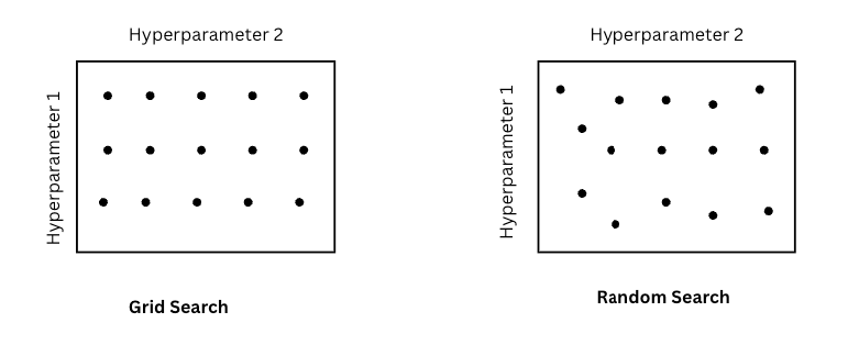
Source: image by author

Grid Search: try every combination on a fixed grid, e.g: Test 5×3 = 15 combinations but only 5 distinct α values
Random Search: sample hyperparameters randomly, e.g: Tests 9 combinations with 9 distinct α values.

Random search is almost always better. If it turns out α matters much more than β, grid search wastes most of its budget testing the same α values repeatedly. Random search naturally explores more values of every hyperparameter regardless of which ones turn out to matter.

Using Random or Grid Search, we can apply Coarse to fine, a multi-round strategy, in which we use random search (or grid search) repeatedly, each time narrowing the search space around the most promising region found in the previous round.

Coarse to fine finds the region of the space that works best, then sample more densely within that region. This focuses compute budget where it matters most.

1.2. Using an Appropriate Scale to pick Hyperparameters

The problem with uniform sampling: sampling hyperparameters uniformly sounds fair, but it isn’t always the right scale for every hyperparameter.

General guidelines:

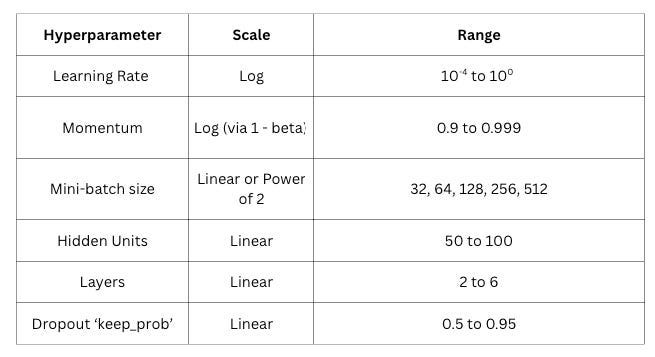
Regarding number of hidden units, sampling uniformly between 50 and 500 makes sense. The difference between 50 and 100 is similar between 50 and 100 is similar in impact to the difference 400 and 450. However, for learning rate, sampling uniformly between 0.0001 and 1 is a terrible idea. 90% of the samples fall between 0.1 and 1, leaving almost nothing exploring the critical low end.

The right scale for learning rate is logarithmic, by which, we can achieve equal probability in each decade from 0.0001 to 1.

# Wrong: Uniform sampling
learning_rate = np.random.uniform(0.0001, 1)
# Correct:
r = -4 * np.random.rand()
learning_rate = 10**r

Similarly, momentum β also needs log scale. β near 1 is particularly sensitive: the difference between β = 0.9 and β = 0.99 is enormous (averaging last 10 vs last 100 gradients), but on a linear scale they look almost identical. The trick is to sample 1 – β on a log scale:

# Sample (1- beta) on log scale
log_val = np.random.uniform(-3, -1)
beta = 1 - 10 ** log_val

1.3. Hyperparameters Tuning in Practice: Pandas vs. Caviar

two fundamentally different approaches to hyperparameter tuning in practice, driven by how much compute you have available.

Panda: we train one model at a time and continuously monitor and adjust it.

Day 1: start training, α = 0.01
Day 2: loss plateauing → increase α to 0.05
Day 3: loss spiking → add momentum
Day 4: overfitting → add dropout

This method is mostly used in:

Limited compute: very large models where a single run takes days or weeks
Fine-tuning large pretrained models

It is used by most practitioners working with large LLMs, where a single training run costs millions of dollars and we can’t afford to run many simultaneously.

Caviar: we train many models simultaneously with different hyperparameter settings and pick the best one:

Model 1: α=0.001, β=0.9 → dev error: 8.2%
Model 2: α=0.01, β=0.9 → dev error: 6.1% ← best
Model 3: α=0.01, β=0.99 → dev error: 7.4%
Model 4: α=0.1, β=0.99 → dev error: 12.3%

This method is mostly used in:

Abundant compute that can run dozens or hundreds of experiments simultaneously
Smaller models where each run takes hours not weeks
Hyperparameter search for production systems where getting the best result matters more than compute cost

It is used by large research labs (Google, Meta) running neural architecture search or systematic hyperparameter sweeps across hundreds of GPUs.

Most practitioners operate somewhere between the two extremes. With modern tools like Weights & Biases sweeps or Ray Tune, we can automate parallel hyperparameter search across multiple GPUs even on a moderate budget — getting some of the benefit of the caviar approach without needing Google-scale infrastructure. But for truly large models, the panda approach that is careful, monitored, intuition-driven tuning remains the dominant paradigm simply because the compute cost of running many experiments is prohibitive.

2. Batch Normalization

2.1. Normalizing Activations in a Networks

You already know that normalizing input features X speeds up training by making the loss landscape more spherical. Batch normalization extends this same idea deeper into the network, by normalizing the activations at each hidden layer so that the inputs to every layer are well-scaled, not just the inputs to the first layer.

The intuition is simple: if normalizing X helps layer 1 train faster, why not also normalize the inputs to layer 2, layer 3, and every layer beyond?

The math is: for a given layer, given the pre-activation values Z:

ε: is a small constant for numerical stability
γ and β are learnable parameters that allow the network to undo the normalization if that’s what the data requires. Without them, every layer would be forced to have 0 mean and unit variance, which may not be optimal for every layer.

Batch norm is typically applied to Z (before the activation) rather than A (after). Normalizing before the activation preserves the nonlinearity’s behavior. If we normalized after ReLU, for example, we’d be distorting the distribution that ReLU just shaped.

2.2. Fitting Batch Norm into a Neural Network

Batch norm is inserted between the linear transformation and the activation function at each layer.

X ──► Z¹ = W¹X + b¹ ──► BN(Z¹) ──► A¹ = g(Z̃¹) ──► Z² ──► BN(Z²) ──► A² ──► ...

Notice that batch norm subtracts the mean, which makes the bias b redundant, since any constant added by b gets subtracted right back out by the mean subtraction. So when using batch norm, biases are dropped and replaced by the learned shift parameter β:

# Without batch norm
Z = W @ A_prev + b      # b matters
# With batch norm
Z = W @ A_prev          # b dropped - β handles the shift
Z_norm = batchnorm(Z)   # normalize
Z_tilde = γ * Z_norm + β  # γ and β are learned instead

Each layer now has two new learnable parameters per neuron, γ (scale) and β (shift), updated via backpropagation alongside W.

Why does Batch Norm Works?

Same as Input normalization: Just as normalizing X makes the loss landscape more spherical for the first layer, normalizing activations does the same for every subsequent layer. Each layer receives inputs in a consistent, well-scaled range, which stabilizes and accelerates training throughout the entire network.
Reduces covariate shift: Covariate shift is when the distribution of inputs to a layer keeps changing as earlier layers update their weights during training. Every time W¹ changes, the distribution of A¹ changes, which means layer 2 is constantly chasing a moving target. Batch norm pins the mean and variance of each layer’s inputs to a stable range, so even as earlier weights change, the distribution seen by later layers stays roughly consistent. Each layer can learn more independently without constantly having to readapt to upstream changes.
Slight regularization effect: Computing mean and variance on a mini-batch introduces noise, each mini-batch gives a slightly different estimate. This noise acts similarly to dropout, adding a mild regularization effect that slightly reduces overfitting. This is a side effect, not the primary purpose: don’t use batch norm as your main regularization strategy.

Batch Norm at Test Time

During training, mean μ and variance σ² are computed per mini-batch. At test time, you often predict one example at a time: there’s no batch to compute statistics over. The solution here is running averages. During training, batch norm tracks exponentially weighted running averages of the mean and variance across all mini-batches

# Updated during training at each mini-batch
running_mean = momentum * running_mean + (1 - momentum) * batch_mean
running_var  = momentum * running_var  + (1 - momentum) * batch_var

At test time, these running averages are frozen and used directly instead of computing batch statistics:

# At test time
Z_norm = (Z - running_mean) / sqrt(running_var + epsilon)
Z_tilde = gamma * Z_norm + beta

This gives stable, deterministic predictions at inference time regardless of batch size, including single-example prediction.

This is handled automatically in PyTorch by using model.eval() after model.train().

In summary:

3. Multi-class Classification

3.1. Softmax Regression

Instead of a single sigmoid neuron at the output, we have C output neurons, one per class. The raw output Z from the final linear layer are fed into the softmax activation function:

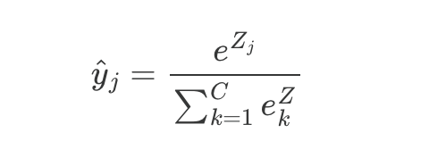
For each output neuron j, softmax divides its exponentiated value by the sum of all exponentiated values. This does 2 things simultaneously: makes al outputs positive (via e^Z) and normalizes them to sum to 1 (via the division).

Example with C = 4:

Z = [2.0, 1.0, 0.1, 0.5]
e^Z = [7.39, 2.72, 1.11, 1.65]    #sum = 12.87
softmax = [0.57, 0.21, 0.09, 0.13]   #sums to 1.0

The network predicts class 1 with 57% probability, class 2 with 21%, and so on. The predicted class is the one with the highest probability, argmax(ŷ).

The e^Z term amplifies differences between logits: a logit that’s slightly larger becomes much larger after exponentiation, making the probability distribution sharper and more decisive. It also ensures all values are positive regardless of the sign of Z.

In the binary case, softmax reduces exactly to logistic regression (sigmoid). Softmax is the generalization of sigmoid to C classes.

3.2. Training a Softmax Classifier

Loss function: cross entropy

For a single example with true label y (a one-hot vector with a 1 in the correct class position):

Since y is one-hot, only one term survives the sum — the log probability of the correct class:

y = [0, 1, 0, 0]       # true class is 2
ŷ = [0.57, 0.21, 0.09, 0.13]
L = -log(0.21) = 1.56   # only the correct class term mattersThe loss is simply how surprised the model is by the correct answer. If the model confidently predicted 0.21 for the true class when it should be near 1.0, the loss is large. To minimize the loss, the model must maximize the probability assigned to the correct class.

The loss is simply how surprised the model is by the correct answer. If the model confidently predicted 0.21 for the true class when it should be near 1.0, the loss is large. To minimize the loss, the model must maximize the probability assigned to the correct class.

Cost function over the full training set

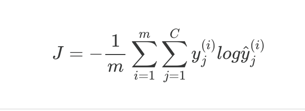
Average cross entropy loss across all m examples and all C classes.

Backpropagation: the gradient

The gradient of the softmax + cross entropy combination is remarkably clearn:

Exactly the same form as logistic regression: the error is just the difference between predicted and true probabilities. This clean gradient is one reason softmax and cross entropy is the standard pairing for multi-class classification.

In PyTorch, CrossEntropyLoss() applies softmax internally.