BERT vs. Transformers: A Complete Architectural and Mathematical Dissection

When I first read about BERT (Bidirectional Encoder Representations from Transformers), the number one question that plagued my mind was a simple definition issue.

We are told BERT is “Bidirectional.” But wait — BERT is based on the Transformer Encoder. In the standard Transformer architecture, the encoder’s self-attention mechanism already attends to every token simultaneously (all-to-all attention). If the underlying architecture is already looking at the whole sentence at once, what is so special or specific about the “Bidirectional” claim in BERT?

Is it just marketing? Is it a fundamental architectural change? Or is it something deeper hidden in the mathematics of how the model is trained?

To answer this, we need to move beyond high-level diagrams and look at the probability modeling, the input structures, and the raw code. This article dissects the difference between the “Transformer Encoder” as a building block and “BERT” as a model.

1. The Transformer: An Architecture, Not a Model

Before we dissect BERT, we must rigorously define what a “Transformer” actually is. It is not a model in itself; it is a parameterized function definition for mapping sequences to sequences.

The original Transformer (Vaswani et al., 2017) consists of two distinct stacks:

1. The Encoder: Processes the input sequence (e.g., a sentence in English).
2. The Decoder: Generates the output sequence (e.g., the translation in French), one token at a time.

The Building Blocks

While they look similar, the Encoder and Decoder have critical differences in their internal layers:

Encoder Layer: Has 2 sub-layers.

1. Multi-Head Self-Attention (sees the whole input).
2. Feed-Forward Network (FFN).

Decoder Layer: Has 3 sub-layers.

1. Masked Multi-Head Self-Attention (can only see past tokens).
2. Cross-Attention (looks back at the Encoder’s output).
3. Feed-Forward Network (FFN).

The core mathematical operation that powers both stacks is Scaled Dot-Product Attention:

Now that we have the full picture, we can see exactly what BERT did: It threw away the Decoder entirely.

2. The Transformer Encoder

BERT is essentially a stack of Transformer Encoders. It completely discards the Decoder and its Cross-Attention mechanism.

A Transformer Encoder takes a sequence of tokens and outputs a sequence of “Contextual Embeddings.”

The Input Representation

The input X to the encoder is a sum of embeddings. In the standard Transformer, this is simply:

• X (Input Representation): The final vector sum fed into the Encoder. It combines “what the word is” with “where the word is.”
• E_{token} (Token Embeddings): The static vector representing the word’s semantic meaning (e.g., “dog” vs. “cat”).
• E_{position} (Position Embeddings): A vector representing the word’s order in the sentence (e.g., Position 0 vs. Position 5), allowing the model to distinguish “Man bites dog” from “Dog bites man.

The “All-to-All” Mechanism

Inside the Encoder, the self-attention mechanism allows every token to attend to every other token.

This means that structurally, the Encoder is already bidirectional. The information flows from the last word to the first word just as easily as it flows forward.

The Conflict: If the Transformer Encoder is already bidirectional, why did the authors of BERT claim “Bidirectionality” was their main contribution? The answer lies not in the architecture, but in the Probability Modeling — specifically, how the model is trained.

3. So, What Is BERT?

BERT is not just “A Transformer Encoder.” It is a Transformer Encoder wrapper with specific Input Modifications and Training Heads.

3.1 The Input Embeddings

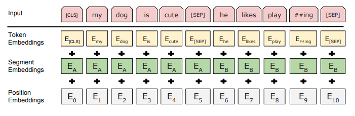
This is a specific differentiator. While a standard Transformer uses Token + Position, BERT uses three distinct embeddings summed together:

• Token Embeddings: The ID of the word (e.g., “Dog” -> 432).
• Position Embeddings: The order in the sequence (e.g., Position 0, Position 1). Note that unlike the original Transformer which used fixed Sine/Cosine functions, BERT uses learned position embeddings.
• Segment Embeddings: This is unique to BERT. It is a learned vector (not just a flag) that tells the model which sentence a token belongs to (Sentence A vs. Sentence B).

3.2 The Training Heads

BERT is trained with two simultaneous heads:

• MLM (Masked Language Modeling) Head: A linear layer + softmax over the vocabulary to predict masked words.
• NSP (Next Sentence Prediction) Head: A binary classification head on the [CLS] token to predict if Sentence B logically follows Sentence A.

The Purpose of the [CLS] Token: BERT inserts a special [CLS] (Classification) token at the very beginning of every input sequence. While other tokens (like “dog”) focus on their local context, the [CLS] token is designed to aggregate the “global understanding” of the entire sequence pair, making it the perfect input for classification tasks.

The NSP Head Detail

The NSP task is a Binary Classification problem. It asks: “Is Sentence B the actual next sentence that followed Sentence A in the original text?”

• Input: The model takes the final hidden state of the [CLS] token from the last transformer layer, denoted as C .

Note: C is simply the 768-dimensional vector representation of the [CLS] token after it has passed through all 12 layers of attention.

• Pooling Layer: The vector C is passed through a dense layer with a Tanh activation.

• Classifier: This projected vector is fed into a simple linear layer that reduces the dimension from 768 to 2.

• Softmax: Finally, a Softmax is applied to get probabilities for P(IsNext). where IsNext is the label “True” (Sentence B is the correct continuation). The alternative label is NotNext (Sentence B is a random sentence from the corpus).

4. Probability Modeling: Where the Real Difference Begins

The difference between GPT, BERT, and a raw Transformer Encoder is not just the layers — it is the Objective Function.

Language modeling is the task of modeling the joint probability distribution of a sequence.

Here, x1, x2, … xn represent the individual tokens (words or sub-words) in a sequence of length $n$Example: In the sentence “AI is the future”, x1=“AI”, x2 = “is”, and xn =“future”.

4.1 Autoregressive Factorization (The GPT Way)

Standard language models (like GPT) factorize this probability from left to right:

To respect this mathematical rule, we must apply a Causal Mask inside the Transformer:

If we allowed the model to see future words (bidirectional attention),

would become trivial (the model would just “cheat” and copy the next word).

4.2 BERT’s Objective: Masked Language Modeling (MLM)

BERT refuses to accept the constraint of looking only to the left. It wants to use the full context (left and right) to understand a word.

Why is this NOT cheating for BERT? If a model can see future words, it would normally just “copy” the answer from the input. BERT solves this by destroying the target information in the input before the model ever sees it.

1. It replaces the target token x_i with [MASK].
2. Even though BERT can see the future tokens, it cannot “copy” the answer because the answer itself has been erased.
3. This forces the model to actually understand the context to fill in the blank.

The loss function sums the log-likelihood of the correct word given the masked context:

The “Train-Test Mismatch” Problem

This masking strategy creates a new problem. If we replace 100% of the selected tokens with [MASK], the model will only ever see [MASK] tokens during training. But in the real world (fine-tuning), there are no [MASK] tokens—only real words. The model might fail because it hasn’t learned to process “normal” sentences.

To bridge this gap, BERT uses a specific 80–10–10 Mixing Rule.

The 80–10–10 Masking Rule

We first select 15% of the tokens in the sequence to be targets. For each selected token, we roll a die independently to decide its fate:

1. 80% of the time: Replace with [MASK]

• Input: The [MASK] is hairy
• Target: dog
• Goal: The standard logic. The model must use the context (“The”, “is”, “hairy”) to guess the missing word.

2. 10% of the time: Replace with a Random Word

• Input: The apple is hairy
• Target: dog
• Goal: This is the “Sanity Check.” The model sees the word “apple”, but its context (“is hairy”) tells it that “apple” is unlikely. This forces the model to verify if the current token fits the context rather than lazily trusting whatever it sees.

3. 10% of the time: Keep the Original Word

• Input: The dog is hairy
• Target: dog
• Goal: This tells the model: “Sometimes, the input is actually correct.” If we only ever masked or randomized words, the model would learn that the input word is always wrong. By keeping it occasionally, we bias the model to trust the input when it matches the context.

Does this explode the training data size?

You might ask: If the 80–10–10 rule creates thousands of possible variations for every sentence (e.g., masking “dog” vs. randomizing “hairy” vs. keeping “dog”), doesn’t our dataset become infinitely large if we try to store them all?

The Answer: It would explode if we pre-generated them and saved them to disk. But we don’t. We use Dynamic Masking.

There is a critical difference between what is stored on the Disk and what happens in Memory:

1. On Disk (Storage): We store only one clean, original copy of the sentence (The dog is hairy). The dataset size remains small.
2. In Memory (Training): The masking is applied on the fly, milliseconds before the data enters the model.

Every time the training loop grabs a batch of sentences, it “rolls the dice” afresh for the 15% of selected tokens.

• Epoch 1: The randomizer selects “dog” and applies the 80% rule (Mask it). The model sees: The [MASK] is hairy.
• Epoch 2: The randomizer selects “dog” again but applies the 10% rule (Randomize it). The model sees: The apple is hairy.

The model never sees the exact same training example twice, effectively training on a dataset of infinite size, while only taking up the storage space of a single book.

5. Step-by-Step Flow: How a Single Example Works

To visualize exactly how the data flows and changes, let’s trace a single training example through the entire BERT pipeline.

Example Sentence Pair:

• Sentence A: “The man went to the store.”
• Sentence B: “He bought a gallon of milk.”
• Label: IsNext (True)

Step 1: Tokenization & Special Tokens

We map words to IDs and add special tokens.

[CLS] the man went to the store [SEP] he bought … [SEP]

Step 2: Segment IDs Assignment

We generate the segment vector indices.

• 0, 0, 0, 0, 0, 0, 0, 0, 1, 1, 1 …
• (0 for Sent A, 1 for Sent B)

Step 3: Masking (The Selection)

We randomly select 15% of indices. Let’s say index 6 (“store”) is selected.

• We apply the 80–10–10 rule. Let’s say it becomes [MASK].
• The input at index 6 is now ID 103 (the ID for [MASK]).

Step 4: Embedding Lookup

The model looks up 3 vectors for every token and sums them:

Step 5: The Transformer Encoder (12 Layers)

This huge matrix (512 * 768) passes through 12 layers of attention.

• Crucial: The [CLS] vector at the start is constantly updating, absorbing context from “man”, “went”, “he”, “milk”.
• Crucial: The [MASK] vector at index 6 is also absorbing context. It looks at “man”, “went”, “he”, “bought” to figure out what it should be.

Step 6: The Outputs (Splitting the Stream)

At the end, we have a final matrix $H^{(12)}$.

• What is this matrix? It is the Hidden State output of the 12th layer.
• Dimensions:

• Content: It contains 512 context-rich vectors.

We split this matrix into two separate jobs:

Job A: Masked LM (Restoring “Store”)

1. Grab the vector at Index 6 ($h_6 in H^{(12)}$).
2. Pass it through the MLM Head (Linear -> LayerNorm -> Linear to Vocab Size).
3. Output: Probability distribution over 30,522 words.
4. Loss: Calculate CrossEntropy between this distribution and the actual word “store”.

Job B: NSP (Checking “IsNext”)

1. Grab the vector at Index 0 ($h_{CLS} in H^{(12)}$).
2. Pass it through the Pooler (Tanh).
3. Pass it through the NSP Head (Linear to 2).
4. Output: [Logit_True, Logit_False].
5. Loss: Calculate CrossEntropy against the true label IsNext.

6. Why BERT Cannot Generate Text Naturally

You might ask: If BERT understands language so well, why can’t I ask it to write a story?

Text generation relies on the chain rule:

You generate word 1, feed it back to get word 2, and so on.

BERT never learned this chain rule. It learned

If you ask BERT to generate, it doesn’t know “what comes next” in a timeline; it only knows “what fits in this hole.” Generating text with BERT requires awkward iterative loops (like masking the next position, predicting it, accepting it, masking the next…) which is computationally expensive and mathematically essentially wrong for the distribution it learned.

7. Real-World Use Cases: What is BERT Actually Used For?

Since BERT cannot generate stories or write code like GPT, what is it good for? It excels at understanding, extracting, and classifying.

7.1 Google Search (Contextual Ranking)

In late 2019, Google announced the biggest update to its search algorithm in years: the integration of BERT.

• Query: “2019 brazil traveler to usa need a visa”
• Pre-BERT: Google ignored the preposition “to.” It saw “Brazil”, “USA”, “Visa” and often returned results for US citizens traveling to Brazil.
• With BERT: The bidirectional attention mechanism understood that “to” indicated a direction. It correctly ranked pages for Brazilian citizens traveling to the US.

Note: BERT does not write the search result snippet; it helps Google retrieve the correct document from the web.

7.2 Extractive Question Answering (SQuAD)

This is the most common misconception. When we say BERT performs “Question Answering,” it does not mean it acts like a Chatbot. It acts like a Highlighter.

• The Task: Given a paragraph (Context) and a Question, find the answer inside the paragraph.
• BERT’s Output: BERT does not generate words. It outputs two integers: a Start Logit and an End Logit.
• Input: “Neil Armstrong was the first man…”
• Question: “Who was the first man?”
• Output: Start_Index: 0, End_Index: 2.
• The Result: The system slices the string from index 0 to 2 and returns “Neil Armstrong.”

If the answer is not explicitly written in the text, BERT cannot answer it.

7.3 Named Entity Recognition (NER)

Identifying and classifying entities in unstructured text.

• Input: “Apple is looking at buying a startup in the UK.”
• BERT:
• Apple to [B-ORG] (Organization)
• UK to [B-LOC] (Location)
• Why BERT? A unidirectional model might see “Apple” and think of the fruit. BERT reads the whole sentence, sees “buying” and “startup,” and correctly classifies “Apple” as a company.

8. Code-Level Differences: Building BERT from Scratch

To prove the difference, let’s implement the core BERT architecture in PyTorch. Notice how we explicitly add the Segment Embeddings and the Masked LM Head, which are not present in a vanilla nn.TransformerEncoder.

Step 1: The Embeddings (The “BERT” Specifics)

import torch
import torch.nn as nn
import math

class BertEmbeddings(nn.Module):
    def __init__(self, vocab_size, max_len=512, hidden_size=768, type_vocab_size=2):
        super().__init__()
        # 1. Token Embeddings (Word Identity)
        self.word_embeddings = nn.Embedding(vocab_size, hidden_size)

        # 2. Position Embeddings (Word Order) - Learned in BERT
        self.position_embeddings = nn.Embedding(max_len, hidden_size)

        # 3. Segment/Token Type Embeddings (Sentence Identity - Specific to BERT)
        self.token_type_embeddings = nn.Embedding(type_vocab_size, hidden_size)

        self.LayerNorm = nn.LayerNorm(hidden_size)
        self.dropout = nn.Dropout(0.1)

    def forward(self, input_ids, token_type_ids):
        seq_length = input_ids.size(1)

        # Generate position IDs dynamically (0, 1, 2, ... seq_len)
        position_ids = torch.arange(seq_length, dtype=torch.long, device=input_ids.device)
        position_ids = position_ids.unsqueeze(0).expand_as(input_ids)

        # Summation of all three embeddings
        embeddings = (self.word_embeddings(input_ids) +
                      self.position_embeddings(position_ids) +
                      self.token_type_embeddings(token_type_ids))

        embeddings = self.LayerNorm(embeddings)
        embeddings = self.dropout(embeddings)
        return embeddings

Step 2: Putting it Together (The BERT Model)

class SimpleBERT(nn.Module):
    def __init__(self, vocab_size, hidden_size=768, num_layers=12, num_heads=12):
        super().__init__()
        self.embeddings = BertEmbeddings(vocab_size, hidden_size=hidden_size)
        
        # Stack of Transformer Encoder Layers
        encoder_layer = nn.TransformerEncoderLayer(
                  d_model=hidden_size, 
                  nhead=num_heads, 
                  batch_first=True, 
                  activation="gelu")
        self.encoder_stack = nn.TransformerEncoder(encoder_layer, num_layers=num_layers)
        
        # The MLM Prediction Head
        self.mlm_head = nn.Sequential(
            nn.Linear(hidden_size, hidden_size),
            nn.GELU(),
            nn.LayerNorm(hidden_size),
            nn.Linear(hidden_size, vocab_size) # Project back to vocab size
        )

        # The NSP Head
        self.nsp_head = nn.Sequential(
            nn.Linear(hidden_size, hidden_size),
            nn.Tanh(),
            nn.Linear(hidden_size, 2)
        )

    def forward(self, input_ids, token_type_ids, attention_mask=None):
        # 1. Get Embeddings
        x = self.embeddings(input_ids, token_type_ids)
        
        # 2. Pass through Encoder Stack
        x = self.encoder_stack(x, src_key_padding_mask=attention_mask)
            
        # 3. Predict masked tokens
        mlm_logits = self.mlm_head(x)
        
        # 4. Predict Next Sentence (Using [CLS] at index 0)
        nsp_logits = self.nsp_head(x[:, 0])
        
        return mlm_logits, nsp_logits

9. Conceptual Summary

To summarize the landscape:

• Transformer: The architecture definition (Attention, Feed-Forward, Normalization).
• Transformer Encoder: A stack of layers allowing full, unmasked self-attention.
• GPT: A Transformer Decoder (masked self-attention) trained to predict the next word.
• BERT: A Transformer Encoder (full self-attention) trained to predict missing words (MLM) and sentence relationships (NSP).

The “Bidirectional” in BERT is not an invention of a new type of neural network layer. It is the successful coupling of an existing bidirectional architecture (the Encoder) with a training objective (MLM) that actually utilizes that bidirectionality without “cheating.”

10. Final Mental Model

Think in layers to debug your understanding:

Level 1 (Mechanism): Scaled Dot-Product Attention.

Note: The core math

is identical in BERT and GPT. The only difference is the Masking Matrix (Causal for GPT, None for BERT).

Level 2 (Architecture): Encoder vs. Decoder.

• BERT uses the Encoder stack.
• Inputs = Token Embeddings + Position Embeddings + Segment Embeddings.

Level 3 (Objective):

• BERT uses a Denoising Objective (Masked LM with 80–10–10 rule).
• GPT uses an Autoregressive Objective (Next Token Prediction).

BERT differs fundamentally at Level 2 and Level 3.

If you understand the attention equations, the need for segment embeddings, and the difference between Autoregressive and Denoising objectives, the distinction between BERT and the Transformer is no longer ambiguous — it is precise.

Thank you for reading! If this article helped clarify the BERT architecture for you, please give it a clap 👏 to help others find it.

References and Further Readings

• BERT Research Paper
• Attention Is All You Need

---

BERT vs. Transformers: A Complete Architectural and Mathematical Dissection was originally published in Towards AI on Medium, where people are continuing the conversation by highlighting and responding to this story.