
Loss Landscapes: Part 1
And why they matter in Machine learning!
TL;DR: In machine learning, the loss landscape is a mathematical surface that maps a model’s parameters (its weights) to a specific “loss” value. The geometry of this surface — which can be full of bowls, ridges, valleys, and saddle points — drastically affects how easy or hard it is to train the model. Even though real-world AI models live in incredibly high dimensions, looking at simple 2D and 3D vizualisations will give you the core intuition you need to understand how AI learns.
What is a loss?
Think of loss as a scorecard that measures how wrong an AI model is. It compares the model’s prediction with the actual, correct answer.
When we calculate loss over an entire dataset, we get a single number. This number is a powerful summary: it tells us exactly how poorly the model is performing.
- The Goal: In machine learning, our main objective is to decrease this loss. A loss of zero would indicate a “perfect” or ideal system that makes zero mistakes.
- The Mechanism: The loss function (sometimes called an objective function) evaluates a specific set of parameters (the input weights assigned to the network). During training, the goal is to tweak and adjust these weights until we find the magic combination where the loss is minimized.
Common Examples of Loss Functions: MSE (Mean Squared Error), Cross-Entropy
NOTE: Different loss functions create different geometric shapes.
Intuition:
1. The Linear Function
You have likely seen a linear function in high school math. It creates a simple, straight line. One example is plotting y = mx (where m is a real number)
2. The Quadratic Function (The Bowl)
When we square the weights (like we do in Mean Squared Error), we get a quadratic function. This forms a beautiful, smooth U-shape or “bowl.”

*This is the holy grail of basic optimization. If you drop a marble anywhere on the sides of this bowl, gravity will pull it down to the single lowest point at the very bottom. In machine learning, that marble is our model, and that bottom point is the perfect set of weights!
3. Other Functions
Real-world loss functions are built using a mix of different math operations.
- Logarithmic and Exponential functions curve rapidly, changing how steeply our “marble” rolls down the hill.

From Loss to Loss Landscapes
So far, we’ve thought about loss in 2D. But how does this translate to a “landscape”?
It all depends on how many parameters (weights) your model has.
- If your model only has one weight, the loss function looks like this: L = f(w). This gives you a simple 2D line graph (like the U-shaped bowl above).
- If your model has two weights, the math looks like this: L = f(w1, w2).
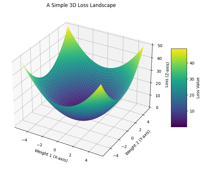
When we have two weights and one loss value, we step into the 3rd dimension! We can now plot this as a 3D surface, which looks exactly like a geographical landscape.
Visualizing the 3D Landscape:
- X-axis: Weight 1
- Y-axis: Weight 2
- Z-axis (Height): The Loss
When you train a model, you are essentially a blindfolded hiker standing somewhere on this 3D mountain range. Your goal is to take steps downhill until you reach the lowest possible valley.
Coding a 3D Loss Landscape
Here is a very simple Python example using matplotlib and numpy to generate and visualize a basic 3D bowl-shaped loss landscape.
import numpy as np
import matplotlib.pyplot as plt
# 1. Define the parameters (Weight 1 and Weight 2)
# We create a grid of numbers from -5 to 5
w1 = np.linspace(-5, 5, 100)
w2 = np.linspace(-5, 5, 100)
W1, W2 = np.meshgrid(w1, w2)
# 2. Define a simple Quadratic Loss Function: L = w1^2 + w2^2
Loss = W1**2 + W2**2
# 3. Plotting the 3D Landscape
fig = plt.figure(figsize=(10, 7))
ax = fig.add_subplot(111, projection='3d')
# Create the surface plot
surface = ax.plot_surface(W1, W2, Loss, cmap='viridis', edgecolor='none')
# Add labels for clarity
ax.set_title('A Simple 3D Loss Landscape')
ax.set_xlabel('Weight 1 (X-axis)')
ax.set_ylabel('Weight 2 (Y-axis)')
ax.set_zlabel('Loss (Z-axis)')
fig.colorbar(surface, shrink=0.5, aspect=5, label='Loss Value')
plt.show()
Output:
4. High vs. Low Dimensional Landscapes
We have looked at models with one or two parameters, but what happens when things get more complex?
The number of dimensions in our loss landscape is directly tied to the number of parameters (weights) our model has:
- 1 parameter creates a 2D curve (a simple line on a graph).
- 2 parameters create a 3D surface (a mountain range we can visualize).
- Many parameters create a high-dimensional surface (a mathematical space that is impossible for the human brain to picture).
Modern neural networks — like the ones powering large language models or image generators — don’t just have one or two parameters. They have millions, and sometimes billions, of parameters. This means their loss landscapes exist in millions of dimensions!
Since we literally cannot visualize a million-dimensional mountain range, data scientists use mathematical tricks to study these complex landscapes in 2D or 3D. We rely on:
- Slices or Projections: Using math to “squash” millions of dimensions down to just two or three while preserving the most important features.
- Contour Plots: Creating a top-down, 2D map of a 3D surface.

5. Convex vs. Non-Convex Landscapes
When data scientists talk about how hard a model is to train, they usually use the words convex and non-convex. This simply describes the overall shape of our loss landscape.
The Convex Landscape (The Easy Path)
A convex landscape is shaped like a perfectly smooth, U-shaped bowl.
- One Minimum: It has exactly one lowest point, which we call the global minimum.
- Easy Optimization: No matter where you randomly start on this landscape, if you just keep walking downhill, you are mathematically guaranteed to reach the absolute best solution.
- Who uses it? Simpler machine learning algorithms, like standard Linear Regression, usually have convex loss landscapes.
The Non-Convex Landscape (The Rugged Terrain)
A non-convex landscape looks less like a smooth bowl and more like a rugged mountain range, complete with hills, valleys, and flat plateaus.
- Multiple Minima: It has many valleys. Some of these are global minima(true bottom), local minima (they look like the bottom because every direction goes up, but they aren’t the absolute lowest point in the whole landscape)
- Saddle Points: It features tricky spots that look flat from one direction (like the bottom of a valley) but slope downward in another direction — exactly like a horse’s saddle.
- Harder Training: Optimization is much harder here. An AI model can easily roll into a local minimum or get stuck on a flat saddle point, thinking it has found the best answer when a much lower valley exists just over the next hill.

* The Deep Learning Reality
NOTE: almost all deep learning models have non-convex landscapes. Because modern neural networks have millions of parameters and complex layers, their loss landscapes are incredibly rugged and chaotic. Finding the absolute best set of weights is often practically impossible. Instead, modern data science is all about finding a “good enough” valley — a local minimum that is low enough for the AI to perform its job well!
Loss Landscapes: Part 1 was originally published in Towards AI on Medium, where people are continuing the conversation by highlighting and responding to this story.