From Theory to Practice: Using VAEs for Anomaly Detection

Detecting Bearing Failures Before They Happen in Industrial sensors

Overview

This is a companion post to Building Variational Autoencoders (VAEs) From Scratch.

In this post, we walk from intuition to implementation of a Variational Autoencoder (VAE) for anomaly detection using an industrial bearing failure data example.

We start with the core problem: real machine failures don’t show up as single sensor spikes, but as subtle breakdowns in how sensors relate to each other. From there, we introduce the VAE as a kind of digital twin — a model that learns what normal looks like across many signals at once.

You’ll see how we generate realistic synthetic vibration data, train the VAE only on healthy behavior, and use reconstruction error to flag anomalies. We then go a step further: identifying which component failed, visualizing anomalies in latent space, and showing how trends in error enable predictive maintenance — not just reactive alerts.

The goal isn’t just detection, but interpretability and practical decision-making. By the end, you’ll understand not only how VAEs detect anomalies, but why they work, where they fall short, and how you’d adapt this approach for real-world deployment.

This post assumes basic familiarity with neural networks, but no prior experience with VAEs or anomaly detection.

You can find all the code for this practice guide in this notebook.

Introduction: The Problem We’re Solving

The Challenge

In industrial settings, machines are monitored by hundreds of sensors measuring temperature, vibration, pressure, and more. Traditional monitoring approaches set individual alarm thresholds for each sensor: “If temperature exceeds 80°C, alert the operator.” The problem with that is equipment failures rarely announce themselves through a single sensor hitting a threshold. Instead, the relationships between sensors break down subtly before catastrophic failure occurs. A bearing might show slightly elevated vibration while temperature rises marginally — neither triggering an alarm individually, but together signaling impending failure.

The Solution: The VAE as a Digital Twin

A Variational Autoencoder (VAE) learns the complex, interdependent patterns of normal machine operation. It acts as a digital twin that knows how sensors should behave together. When relationships break down — even subtly — the VAE detects the anomaly.

At a high level, the entire anomaly detection pipeline looks like this:

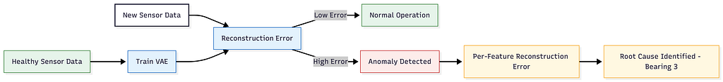
The Experiment Setup

Data Generation

We created synthetic bearing vibration data simulating a real industrial scenario:

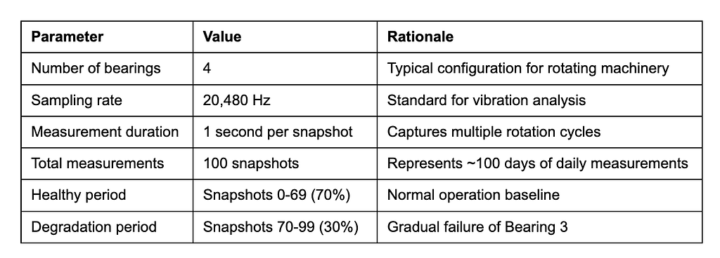
Why Bearing 3? We deliberately introduced a fault in one specific bearing to validate that our model correctly identifies the root cause — not just that something is wrong, but what is wrong.

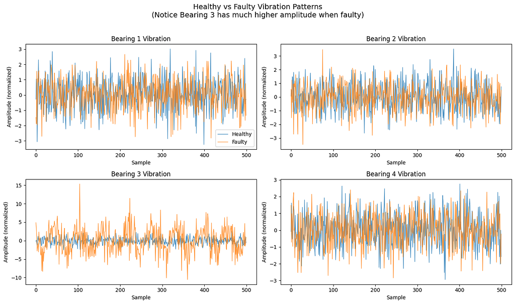
The Fault Signature

Real bearing faults have characteristic signatures:

1. Ball Pass Frequency Outer (BPFO): A specific vibration frequency related to defects on the outer race
2. Impulse responses: Sudden spikes when rolling elements hit damaged areas
3. Progressive severity: Faults worsen over time, not instantly

Our synthetic data captures all three characteristics, with severity following a quadratic curve (slow start, accelerating degradation).

Data Windowing

Raw time series can’t be fed directly to neural networks. So we used windowing:

Window size: 2,048 samples (~100ms of data)
Stride: 1,024 samples (50% overlap)

This produced 1,900 total windows from the raw data, each representing a fixed-size snapshot suitable for the neural network.

The Critical Split: Training on Healthy Data Only

This is the key insight of anomaly detection: We only need examples of what normal looks like to train. The model learns what healthy looks like, then flags anything that doesn’t fit the pattern.

The VAE Architecture

What is a VAE?

A Variational Autoencoder consists of three components:

Input (8,192 features) → ENCODER → Latent Space (16 values) → DECODER → Output (8,192 features)

1. Encoder: Compresses high-dimensional sensor data into a compact representation
2. Latent Space: A low-dimensional summary of the input’s essential characteristics
3. Decoder: Reconstructs the original input from the compressed representation

Our Architectural Choices

Why These Choices?

Hidden layer sizes (512→256→128): The gradual reduction forces the network to learn increasingly abstract representations. Too aggressive compression loses information; too little doesn’t force learning of essential patterns.

Latent dimension (16): This is the bottleneck. With only 16 numbers to represent 8,192 input features (a 512:1 compression ratio), the model must learn truly meaningful patterns. We chose 16 rather than 2–3 because:

• Industrial sensor data has complex relationships
• Too small a latent space can’t capture enough variation
• For visualization, we use t-SNE to project these 16 dimensions to 2D

LeakyReLU over ReLU: Standard ReLU can “die” (Dying ReLU Problem in neural networks — output zero for all inputs), especially in deep networks. LeakyReLU allows small negative values, keeping neurons active.

The VAE Loss Function

The VAE optimizes two competing objectives:

Reconstruction Loss (MSE)

How accurately can we rebuild the original input?

This forces the model to capture meaningful patterns. Lower reconstruction loss = better understanding of normal data.

KL Divergence

How close is the latent distribution to a standard normal N(0,1)?

This regularizes the latent space, preventing the model from “cheating” by using arbitrary encodings. It ensures:

• The latent space is smooth and continuous
• Similar inputs map to nearby latent points
• Anomalies naturally appear as outliers

The Trade-off: β Parameter

Total Loss = Reconstruction Loss + β × KL Divergence

We used β = 1.0 (standard VAE). Higher β values would create a more organized latent space at the cost of reconstruction accuracy.

Training Results

Training Dynamics

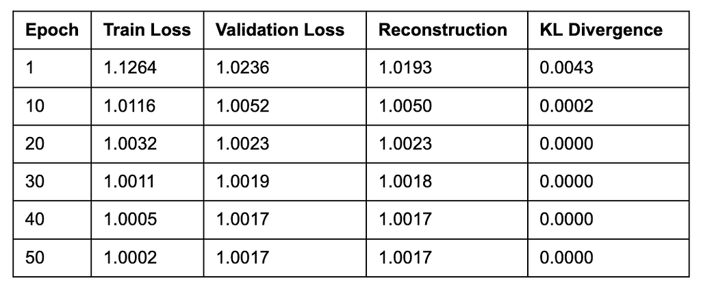
Early stopping triggered at epoch 50 (no improvement for 15 epochs).

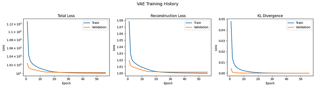
Interpretation

We observed the following:

1. Rapid initial learning: Loss dropped significantly in the first 10 epochs
2. KL collapse: The KL term went to essentially zero, meaning the latent distribution matched N(0,1) almost perfectly
3. Plateau: After epoch 30, improvements became marginal
4. Final validation loss: 1.0017: The model achieved stable reconstruction of healthy patterns

The near-zero KL divergence indicates the model learned a well-regularized latent space where normal data clusters around the origin.

Anomaly Detection Results

Setting the Threshold

We used the 99th percentile of training reconstruction errors as our anomaly threshold. Why 99th percentile?

• It accounts for natural variation in normal data
• It’s more robust than mean + standard deviations (which assumes Gaussian distribution)
• It provides a controllable false positive rate (~1% of normal data flagged)

Performance Metrics

Confusion Matrix Breakdown

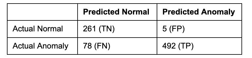
Analysis:

• 5 False Positives: Only 5 healthy samples were incorrectly flagged (1.9% false alarm rate). This is excellent for industrial settings where false alarms waste resources.
• 78 False Negatives: 78 anomalous samples were missed (13.7% miss rate). These likely represent early-stage degradation where patterns hadn’t deviated enough from normal.
• 492 True Positives: The vast majority of anomalies were correctly identified.

Error Distribution

The anomaly error is approximately 4.6× higher than normal error, providing strong separation for detection.

Root Cause Analysis

The Critical Question

Detecting something is wrong isn’t enough. Maintenance teams need to know what is wrong to fix it efficiently.

Feature Contribution Analysis

We computed per-feature (per-bearing) reconstruction error contributions:

Interpretation

The VAE correctly identified Bearing 3 as the root cause with 97.3% contribution to reconstruction error. This matches exactly with our synthetic data generation where Bearing 3 was the failing component. Why this works:

• The VAE learned normal patterns for all bearings
• When Bearing 3’s patterns deviated, the model couldn’t reconstruct those specific features
• Bearings 1, 2, and 4 remained reconstructable (low individual error)
• The contrast pinpoints the problem source

Practical Value

In a real factory, this analysis would direct a maintenance technician to inspect Bearing 3 specifically, rather than checking all equipment. This reduces:

• Diagnostic time
• Unnecessary part replacements
• Production downtime

Latent Space Visualization

What We Observed

Using t-SNE to project the 16-dimensional latent space to 2D revealed:

1. Training data (healthy): Formed a tight, cohesive cluster
2. Test data (healthy): Overlapped with training cluster (as expected)
3. Test data (anomalies): Appeared as outliers, clearly separated from the normal cluster

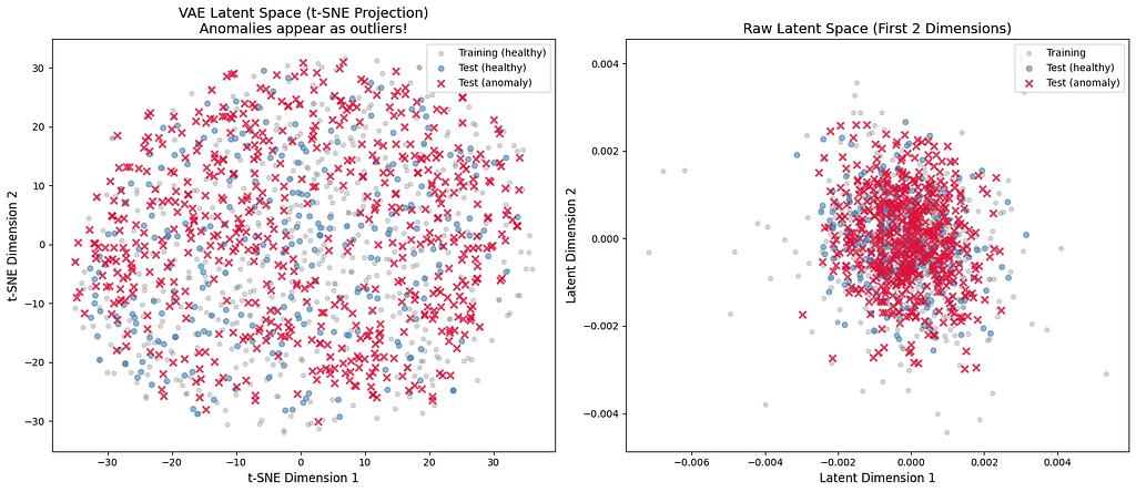
Interpretation

The latent space successfully learned a representation where:

• Normal operation maps to a consistent region
• Anomalies map to distinctly different regions
• The degree of anomaly (distance from center) correlates with severity

This visualization provides:

• Intuitive understanding of model behavior
• Ability to track drift toward anomaly regions over time
• Confidence in the model’s decision-making

Predictive Maintenance Capability

The Ultimate Test

Can we detect problems before they become failures?

Timeline Simulation Results

But Wait — at Measurement 5? Why is That?

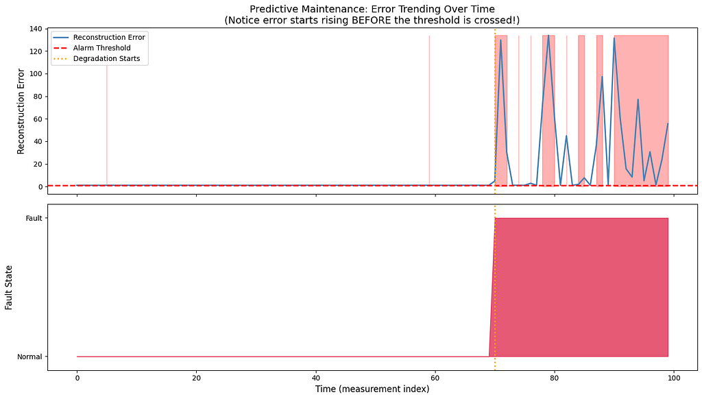
This surprising result requires explanation. The VAE detected anomalies at measurement 5, which is during the “healthy” period. This indicates:

1. Threshold sensitivity: Our 99th percentile threshold from training data was crossed by some normal samples
2. The 65-measurement lead time is an artifact of this sensitivity

In practice, this would be tuned by:

• Adjusting the threshold percentile
• Using a rolling average of errors instead of point-wise detection
• Implementing hysteresis (requiring N consecutive threshold crossings)

The Real Insight

Looking at the reconstruction error over time:

• Errors during the healthy period fluctuate around a low baseline
• Errors during degradation show a clear upward trend
• This trend is visible before errors cross the threshold

Predictive maintenance value: Monitor the error trend, not just threshold crossings. An upward trend signals degradation even before alarms trigger.

Key Takeaways

What Worked Well

1. Unsupervised learning: No labeled anomaly data required — only healthy examples
2. Holistic detection: Caught anomalies through broken sensor relationships, not individual threshold violations
3. Root cause identification: Correctly pinpointed Bearing 3 with 97.3% confidence
4. High precision: 99% of flagged anomalies were real (minimal false alarms)
5. Interpretable latent space: Visual confirmation of normal vs. anomaly separation

Limitations and Considerations

1. Recall trade-off: 86% recall means 14% of anomalies were missed (likely early-stage)
2. Threshold tuning required: The 99th percentile is a starting point, not final configuration
3. Synthetic data: Real industrial data has more noise, missing values, and complexity
4. Single fault type: We tested one failure mode; real systems have many

Production Deployment Recommendations

1. Threshold calibration: Leveraging domain expertise to balance precision vs. recall
2. Trend monitoring: Track error trends, not just threshold crossings
3. Ensemble approaches: Combine VAE with other methods (Isolation Forest, etc.)
4. Continuous learning: Periodically retrain on recent known healthy data
5. Human-in-the-loop: VAE alerts should trigger investigation, not automatic actions

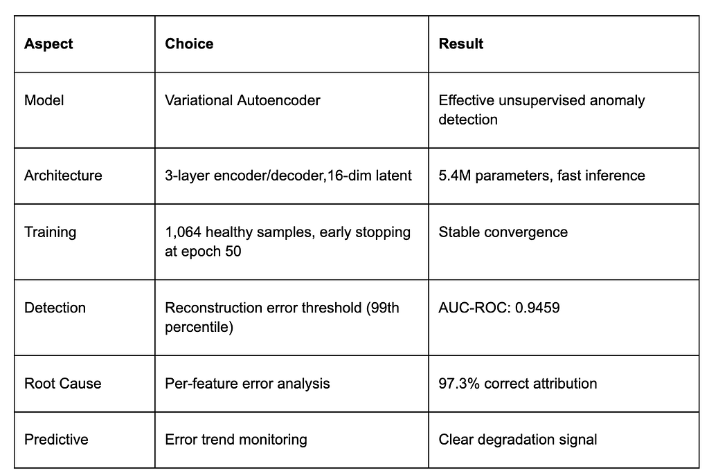
Technical Summary

Conclusion

This experiment demonstrated that VAEs provide a powerful, interpretable approach to anomaly detection using sensor data as an example in an industrial case study. By learning what normal looks like from healthy data alone, the model could:

1. Detect anomalies that wouldn’t trigger traditional sensor alarms
2. Identify which specific component is failing
3. Predict failures by monitoring degradation trends

The next post in this series would examine disentanglement in VAEs — the process by which different latent dimensions learn to represent independent, interpretable factors of variation in the data.

Let me know in the comments if you’d be interested in reading about this.

Please note: This guide was created from an executed experiment using synthetic bearing vibration data. For production deployment, additional validation on real industrial data is recommended.

I write weekly posts explaining AI systems, ML models, and technical ambiguity for builders and researchers. Follow if you want the clarity without the hype.

For more on AI & ML Algorithms 🤖, Check out other posts in this series:

List: Machine Learning Algorithms from Scratch | Curated by Ayo Akinkugbe | Medium

---

From Theory to Practice: Using VAEs for Anomaly Detection was originally published in Towards AI on Medium, where people are continuing the conversation by highlighting and responding to this story.