: Demystifying Gradient Descent from Scratch")
Beyond model.fit(): Demystifying Gradient Descent from Scratch
In the real world, running from sklearn.linear_model import SGDRegressor and calling model.fit(X, y) is easy. But what happens when your model doesn’t converge? What happens when your loss explodes to infinity? If you treat your algorithms like a “Black Box,” you’ll be stuck. Today, we are opening that box. We are going to build Gradient Descent (Batch, Stochastic, and Mini-Batch) entirely from scratch using pure Python and NumPy.
🧮 The Mathematical Foundation
Before we write a single line of code, we need to understand what we are optimizing. The goal of Linear Regression is to minimize the error between our predicted values and the actual values. We use the Mean Squared Error (MSE) as our Loss Function (L):

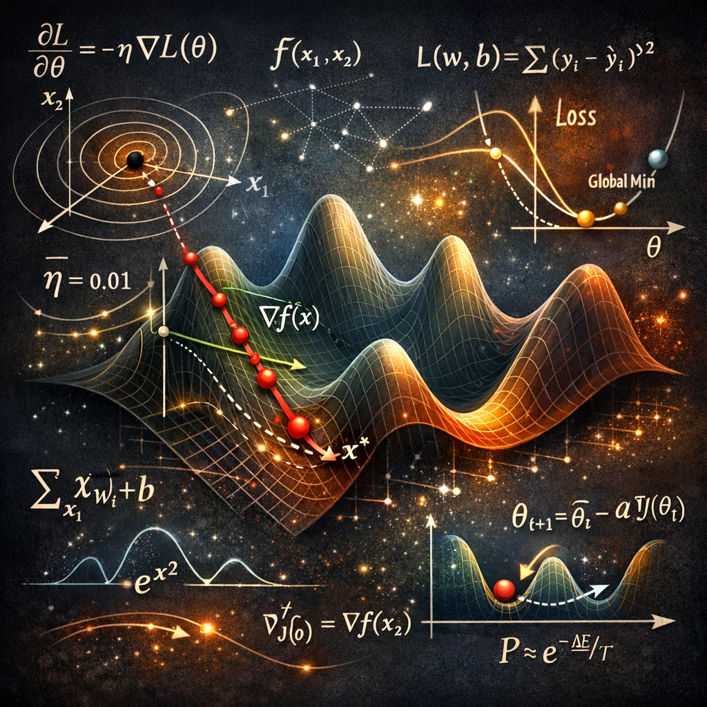
Gradient Descent is an iterative optimization algorithm. Imagine you are blindfolded on a mountain and want to reach the lowest point (the minimum error). You feel the slope of the ground beneath your feet and take a step in the steepest downward direction.
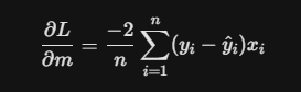
To find that “slope,” we take the partial derivatives of our Loss Function with respect to our intercept b and our coefficients/slopes m:
For the Intercept (b):

For the Coefficients (m):
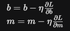
We then update our weights using a Learning Rate (n), which dictates the size of the step we take down the mountain:
💻 Code Implementation (From Scratch)
Let’s translate these mathematical concepts into pure Python. We will look at the three main variants of Gradient Descent.
1. Batch Gradient Descent
Batch GD calculates the error for the entire training dataset before making a single update to the weights. It’s stable and produces a smooth path to the minimum, but it is incredibly slow and computationally expensive for massive datasets.
- How it Works: In the GDRegressor.fit method, Y_hat is calculated using the full X_train matrix. The gradients (intercept_der and coef_der) are then derived from the mean error of every single data point in the training set.
- The Path: It takes a very direct, smooth path toward the minimum. Because it uses the average gradient of the whole population, it never “gets distracted” by outliers in a single step.
- The Downside: Memory is the bottleneck. If you have 10 million rows, your RAM must hold that entire matrix to perform a single update. It is computationally “expensive” per iteration.
import numpy as np
class GDRegressor:
    def __init__(self, Learning_Rate, Epochs):
        self.Learning_Rate = Learning_Rate
        self.Epochs = Epochs
        self.coef = None
        self.intercept = None
        self.loss_history = []
    def fit(self, X_train, Y_train):
        self.intercept = 0
        self.coef = np.ones(X_train.shape[1])
        for i in range(self.Epochs):
            # Calculate predictions for the ENTIRE batch
            Y_hat = np.dot(X_train, self.coef) + self.intercept
            loss = np.mean((Y_train - Y_hat) ** 2)
            self.loss_history.append(loss)
            # Calculate gradients
            intercept_der = -2 * np.mean(Y_train - Y_hat)
            coef_der = -2 * np.dot((Y_train - Y_hat), X_train) / X_train.shape[0]

            # Update weights
            self.intercept -= self.Learning_Rate * intercept_der
            self.coef -= self.Learning_Rate * coef_der
    def predict(self, X_test):
        if self.coef is not None:
            return np.dot(X_test, self.coef) + self.intercept
    def r2_score(self, Y_true, Y_pred):
        ss_total = np.sum((Y_true - Y_true.mean()) ** 2)
        ss_res = np.sum((Y_true - Y_pred) ** 2)
        return 1 - (ss_res / ss_total)
2. Stochastic Gradient Descent (SGD)
When dealing with “Big Data,” calculating the gradient over millions of rows for a single step is impossible. SGD solves this by updating the parameters for every single random training sample. It’s extremely fast but results in a highly erratic, noisy path to the minimum.
- How it Works: In the SGDRegressor.fit method, a nested loop iterates through the number of samples. For every iteration, it picks one random index (idx) and immediately updates the intercept and coef based solely on that one point’s error.
- The Path: The path to the minimum is “noisy” and looks like a zigzag. Because it only sees one point at a time, it might jump in the wrong direction if it hits an outlier. However, this “noise” can actually be a benefit, as it helps the model “jump out” of local minima in non-convex landscapes.
- The Upside: It is extremely fast and can handle “online learning” where data arrives in a continuous stream. You don’t need to load the whole dataset into memory.
- The Downside: It works well on the large dataset but if there is no decaying learning rate then it oscillates around the center
class SGDRegressor:
    def __init__(self, Learning_Rate, Epochs):
        self.Learning_Rate = Learning_Rate
        self.Epochs = Epochs
        self.coef = None
        self.intercept = None
    def fit(self, X_train, Y_train):
        self.intercept = 0
        self.coef = np.ones(X_train.shape[1])
        for i in range(self.Epochs):
            for j in range(X_train.shape[0]):
                # Pick ONE random sample
                idx = np.random.randint(0, X_train.shape[0])
                Y_hat = np.dot(X_train[idx], self.coef) + self.intercept

                # Gradients for the single sample
                intercept_der = -2 * (Y_train[idx] - Y_hat)
                coef_der = -2 * np.dot((Y_train[idx] - Y_hat), X_train[idx])

                # Immediate update
                self.intercept -= self.Learning_Rate * intercept_der
                self.coef -= self.Learning_Rate * coef_der
    def predict(self, X_test):
        if self.coef is not None:
            return np.dot(X_test, self.coef) + self.intercept
Note: Because SGD is so volatile near the minimum, we often use Learning Schedules (decaying the learning rate over time) so the algorithm can settle rather than bounce around endlessly.
3. Mini-Batch Gradient Descent
This is the gold standard used in Deep Learning. Instead of 1 sample (SGD) or all samples (Batch), we take a small chunk (e.g., 32, 64, or 128 rows). It leverages vectorized matrix operations while still being memory efficient.
- How it Works: The MBGDRegressor takes a batch_size parameter (commonly 32, 64, or 128). In each epoch, it selects a random sample of indices of that size and calculates the gradient for that specific subset.
- The Path: It is significantly smoother than SGD because the “noise” is averaged out over the batch, but it remains much faster than Batch GD because it doesn’t wait to see the whole dataset.
- The Secret Weapon (Vectorization): MBGD allows us to use highly optimized matrix multiplication (NumPy/BLAS) on the GPU or CPU. A batch of 64 is often processed almost as fast as a single data point due to parallelization.
import random

class MBGDRegressor:
    def __init__(self, batch_size, Learning_Rate, Epochs):
        self.Learning_Rate = Learning_Rate
        self.Epochs = Epochs
        self.coef = None
        self.intercept = None
        self.batch_size = batch_size

    def fit(self, X_train, Y_train):
        self.intercept = 0
        self.coef = np.ones(X_train.shape[1])

        for i in range(self.Epochs):
            # Iterate through the number of batches
            for j in range(int(X_train.shape[0]/self.batch_size)):

                # Sample a batch
                idx = random.sample(range(0, X_train.shape[0]), self.batch_size)

                Y_hat = np.dot(X_train[idx], self.coef) + self.intercept

                intercept_der = -2 * np.mean(Y_train[idx] - Y_hat)
                coef_der = -2 * np.dot((Y_train[idx] - Y_hat), X_train[idx])

                self.intercept -= self.Learning_Rate * intercept_der
                self.coef -= self.Learning_Rate * coef_der

    def predict(self, X_test):
        if self.coef is not None:
            return np.dot(X_test, self.coef) + self.intercept
1. Feature Scaling (The Silent Killer)
- The Assumption: All features are on a similar numerical scale.
- Consequences: If Feature A ranges from 0–1 and Feature B ranges from 0–10,000, the contour plot of your loss function becomes an elongated, stretched oval. Gradient Descent will endlessly oscillate back and forth across the narrow valley and take forever to converge.
- Detection: Simply run .describe() on your Pandas dataframe. If the max and min vastly differ across columns, you have a scaling problem.
- Remedy: Always apply StandardScaler (Z-score normalization) or MinMaxScaler before fitting a GD model.
2. Convexity of the Loss Function
- The Assumption: The error landscape is a clean “bowl” shape with only one lowest point.
- Consequences: While MSE in Linear Regression is strictly convex (meaning any local minimum is the global minimum), if you use complex neural networks or non-convex loss functions, your model might get trapped in a local minimum and fail to find the best weights.
- Remedy: For non-convex problems, using Mini-Batch SGD with Momentum or advanced optimizers like RMSProp, Adagrad, Adam helps punch through local minima.
3. Appropriate Learning Rate Selection
- The Assumption: The learning rate n is perfectly balanced.
- Consequences: If n is too small, your model might take days to train. If n is too large, you will overshoot the minimum, and your loss will mathematically explode to NaN or infinity.
- Detection: Plot your Loss vs. Epochs curve.
- Remedy: Use Grid Search to find the optimal n, or implement learning schedules (e.g., halving the learning rate every 10 epochs).
📉 Visual Interpretation Guide: Seeing Your Algorithm Work
To truly master Gradient Descent, you cannot rely solely on the final R² score. You must visualize the learning process. These plots are the “pulse” of your model — they tell you if your learning rate is healthy or if your model is fundamentally broken.
1. The “Good” vs. “Bad” Loss Curve
The first thing every engineer should check is the Loss vs. Epochs plot. This tells you how effectively the model is minimizing error over time.
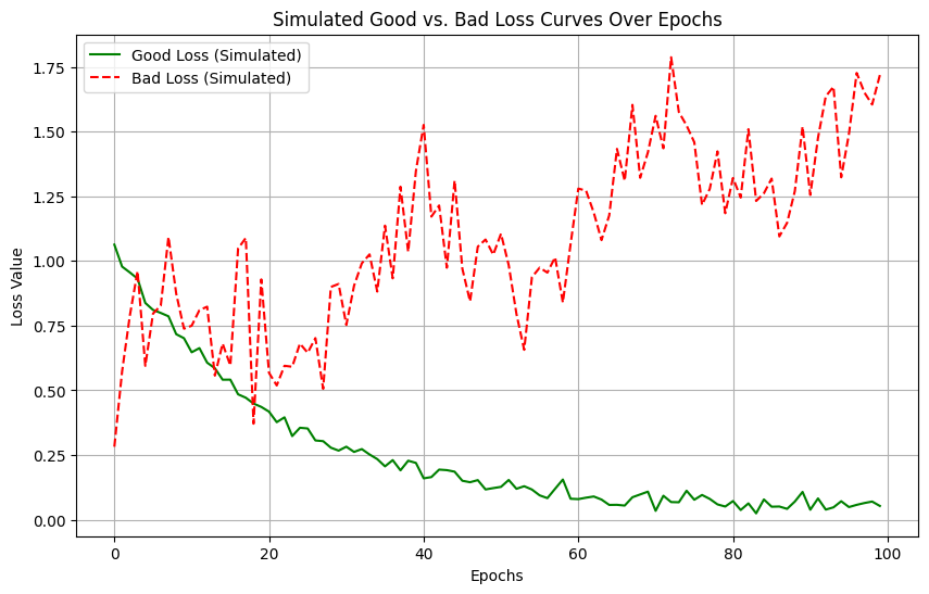

- The “Good” Plot (Smooth Decay, Green Line): As seen in the left panel of the first image, a well-tuned Gradient Descent shows a steep drop in MSE during the first few epochs. This is where the model makes “big gains” by moving from random initialization toward the general area of the minimum. Over time, the curve flattens out (plateaus), indicating that the model has converged and further training won’t yield significant improvements.
- The “Bad” Plot (Divergence/Explosion, Red Line): The right panel (shown on a log scale) illustrates what happens when your Learning Rate (n{eta}) is too high. Instead of settling into the valley of minimum error, the model overshoots it so violently that it lands further away on the other side. This creates a feedback loop where the error grows exponentially. If you see your loss becoming NaN or a massive number, your learning rate is the culprit.
2. Contour Paths: The Geometry of Optimization
If we look at the 2D parameter space (Intercept b vs. Coefficient m), we can map the “path” the algorithm takes down the error mountain.
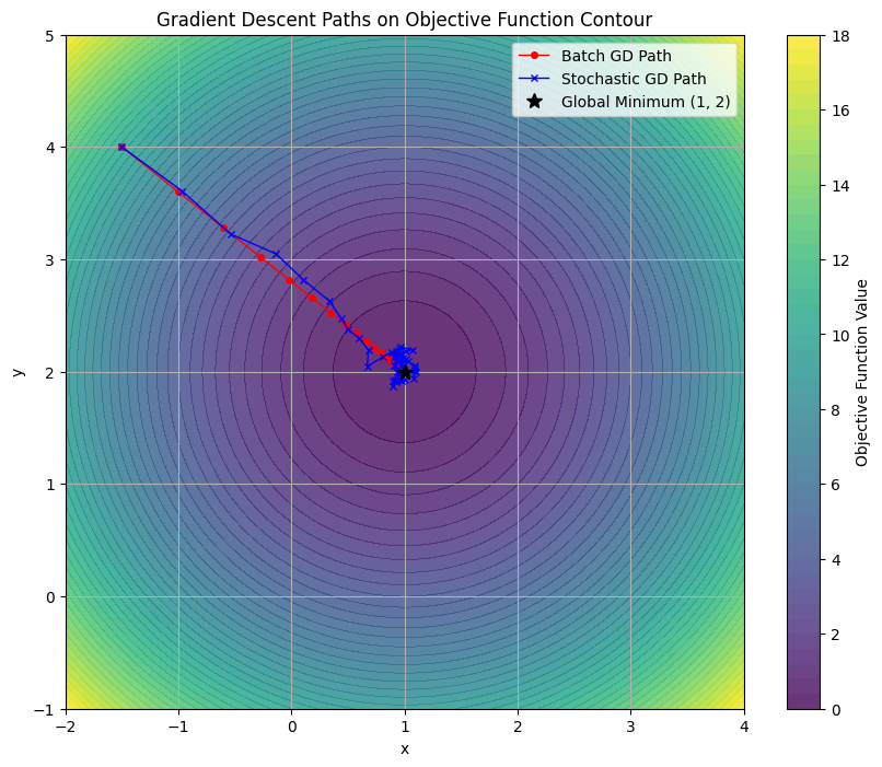
- Batch Gradient Descent (Red Path): Notice how the red line is smooth and moves almost perpendicularly to the contour lines. Because it averages the gradient across the entire dataset, it knows the “true” direction of the steepest descent. It is slow but incredibly precise, moving like a calculated hiker toward the global minimum (the black star).
- Stochastic Gradient Descent (Blue Path): The Blue path looks like a “drunken walk.” Because it updates the weights after seeing only one random data point, it is constantly being tugged in slightly different directions. While it eventually reaches the same neighborhood as the global minimum, it never truly “settles” and instead continues to dance around the target. This noise, however, is exactly what allows it to be computationally fast and escape flat regions of the loss landscape.
✉ Let’s Connect!
Mastering these visual and mathematical foundations is the first step toward becoming a robust Data Scientist.
- LinkedIn: pruthil-prajapati
- Email: Gmail
- GitHub: Pruthil-2910
Keep exploring the math behind the models!
#BuildInPublic #ArtificialIntelligence #DataEngineering #SoftwareEngineering #Mathematics #ProgrammingTips #100DaysOfCode #UnderTheHood #MathForML #FromScratch #CodeNewbie #Vectorization #Optimization #AlgorithmDesign #NumPy
🚀 Beyond model.fit(): Demystifying Gradient Descent from Scratch was originally published in Towards AI on Medium, where people are continuing the conversation by highlighting and responding to this story.