TF-IDF vs. Embeddings: From Keywords to Semantic Search

---

---

TF-IDF vs. Embeddings: From Keywords to Semantic Search

In this tutorial, you’ll learn what vector databases and embeddings really are, why they matter for modern AI systems, and how they enable semantic search and retrieval-augmented generation (RAG). You’ll start from text embeddings, see how they map meaning to geometry, and finally query them for similarity search — all with hands-on code.

This lesson is the 1st of a 3-part series on Retrieval Augmented Generation:

1. TF-IDF vs. Embeddings: From Keywords to Semantic Search (this tutorial)
2. Lesson 2
3. Lesson 3

To learn how to build your own semantic search foundation from scratch, just keep reading.

---

Series Preamble: From Text to RAG

Before we start turning text into numbers, let’s zoom out and see the bigger picture.

This 3-part series is your step-by-step journey from raw text documents to a working Retrieval-Augmented Generation (RAG) pipeline — the same architecture behind tools such as ChatGPT’s browsing mode, Bing Copilot, and internal enterprise copilots.

By the end, you’ll not only understand how semantic search and retrieval work but also have a reproducible, modular codebase that mirrors production-ready RAG systems.

---

What You’ll Build Across the Series

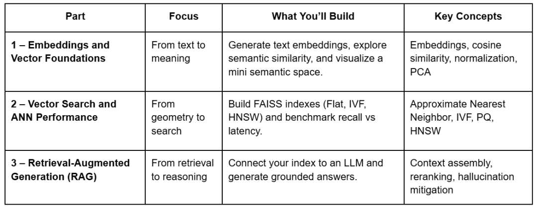
Each lesson builds on the last, using the same shared repository. You’ll see how a single set of embeddings evolves from a geometric curiosity into a working retrieval system with reasoning abilities.

---

Project Structure

Before writing code, let’s look at how the project is organized.

All 3 lessons share a single structure, so you can reuse embeddings, indexes, and prompts across parts.

Below is the full layout — the files marked with Part 1 are the ones you’ll actually touch in this lesson:

vector-rag-series/
├── 01_intro_to_embeddings.py          # Part 1 – generate & visualize embeddings
├── 02_vector_search_ann.py            # Part 2 – build FAISS indexes & run ANN search
├── 03_rag_pipeline.py                 # Part 3 – connect vector search to an LLM
│
├── pyimagesearch/
│   ├── __init__.py
│   ├── config.py                      # Paths, constants, model name, prompt templates
│   ├── embeddings_utils.py            # Load corpus, generate & save embeddings
│   ├── vector_search_utils.py         # ANN utilities (Flat, IVF, HNSW)
│   └── rag_utils.py                   # Prompt builder & retrieval logic
│
├── data/
│   ├── input/                         # Corpus text + metadata
│   ├── output/                        # Cached embeddings & PCA projection
│   ├── indexes/                       # FAISS indexes (used later)
│   └── figures/                       # Generated visualizations
│
├── scripts/
│   └── list_indexes.py                # Helper for index inspection (later)
│
├── environment.yml                    # Conda environment setup
├── requirements.txt                   # Dependencies
└── README.md                          # Series overview & usage guide

In Lesson 1, we’ll focus on:

• config.py: centralized configuration and file paths
• embeddings_utils.py: core logic to load, embed, and save data
• 01_intro_to_embeddings.py: driver script orchestrating everything

These components form the backbone of your semantic layer — everything else (indexes, retrieval, and RAG logic) builds on top of this.

---

Why Start with Embeddings

Everything begins with meaning. Before a computer can retrieve or reason about text, it must first represent what that text means.

Embeddings make this possible — they translate human language into numerical form, capturing subtle semantic relationships that keyword matching cannot.

In this 1st post, you’ll:

• Generate text embeddings using a transformer model (sentence-transformers/all-MiniLM-L6-v2)
• Measure how similar sentences are in meaning using cosine similarity
• Visualize how related ideas naturally cluster in 2D space
• Persist your embeddings for fast retrieval in later lessons

This foundation will power the ANN indexes in Part 2 and the full RAG pipeline in Part 3.

With the roadmap and structure in place, let’s begin our journey by understanding why traditional keyword search falls short — and how embeddings solve it.

---

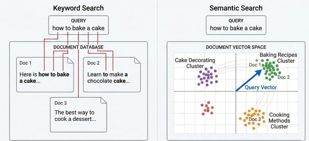
The Problem with Keyword Search

Before we talk about vector databases, let’s revisit the kind of search that dominated the web for decades: keyword-based retrieval.

Most classical systems (e.g., TF-IDF or BM25) treat text as a bag of words. They count how often words appear, adjust for rarity, and assume overlap = relevance.

That works… until it doesn’t.

---

When “Different Words” Mean the Same Thing

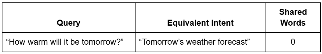
Let’s look at 2 simple queries:

Q1: “How warm will it be tomorrow?”

Q2: “Tomorrow’s weather forecast”

These sentences express the same intent — you’re asking about the weather — but they share almost no overlapping words.

A keyword search engine ranks documents by shared terms.

If there’s no shared token (“warm,” “forecast”), it may completely miss the match.

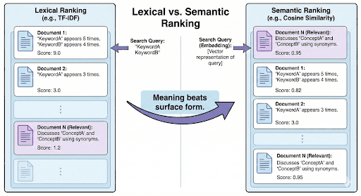
This is called an intent mismatch: lexical similarity (same words) fails to capture semantic similarity (same meaning).

Even worse, documents filled with repeated query words can falsely appear more relevant, even if they lack context.

---

Why TF-IDF and BM25 Fall Short

TF-IDF (Term Frequency–Inverse Document Frequency) gives high scores to words that occur often in one document but rarely across others.

It’s powerful for distinguishing topics, but brittle for meaning.

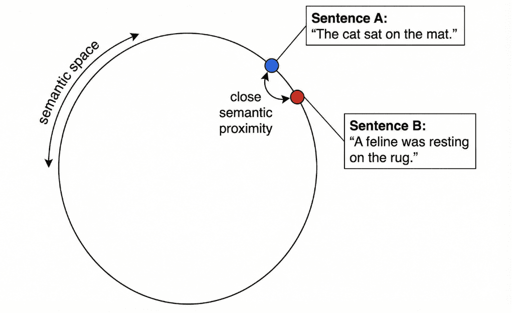
For example, in the sentence:

“The cat sat on the mat,”
TF-IDF only knows about surface tokens. It cannot tell that “feline resting on carpet” means nearly the same thing.

BM25 (Best Matching 25) improves ranking via term saturation and document-length normalization, but still fundamentally depends on lexical overlap rather than semantic meaning.

---

The Cost of Lexical Thinking

Keyword search struggles with:

• Synonyms: “AI” vs “Artificial Intelligence”
• Paraphrases: “Fix the bug” vs “Resolve the issue”
• Polysemy: “Apple” (fruit) vs “Apple” (company)
• Language flexibility: “Movie” vs “Film”

For humans, these are trivially related. For traditional algorithms, they are entirely different strings.

Example:

Searching “how to make my code run faster” might not surface a document titled “Python optimization tips” — even though it’s exactly what you need.

---

Why Meaning Requires Geometry

Language is continuous; meaning exists on a spectrum, not in discrete word buckets.

So instead of matching strings, what if we could plot their meanings in a high-dimensional space — where similar ideas sit close together, even if they use different words?

That’s the leap from keyword search to semantic search.

Instead of asking “Which documents share the same words?” we ask:

“Which documents mean something similar?”

And that’s precisely what embeddings and vector databases enable.

Now that you understand why keyword-based search fails, let’s explore how vector databases solve this — by storing and comparing meaning, not just words.

---

What Are Vector Databases and Why They Matter

Traditional databases are great at handling structured data — numbers, strings, timestamps — things that fit neatly into tables and indexes.

But the real world isn’t that tidy. We deal with unstructured data: text, images, audio, videos, and documents that don’t have a predefined schema.

That’s where vector databases come in.

They store and retrieve semantic meaning rather than literal text.

Instead of searching by keywords, we search by concepts — through a continuous, geometric representation of data called embeddings.

---

The Core Idea

Every piece of unstructured data — such as a paragraph, image, or audio clip — is passed through a model (e.g., a SentenceTransformer or CLIP (Contrastive Language-Image Pre-Training) model), which converts it into a vector (i.e., a list of numbers).

These numbers capture semantic relationships: items that are conceptually similar end up closer together in this multi-dimensional space.

Example:
“vector database,” “semantic search,” and “retrieval-augmented generation” might cluster near each other, while “weather forecast” or “climate data” form another neighborhood.

Formally, each vector is a point in an N-dimensional space (where N = model’s embedding dimension, e.g., 384 or 768).

The distance between points represents how related they are — cosine similarity, inner product, or Euclidean distance being the most common measures.

---

Why This Matters

The beauty of vector databases is that they make meaning searchable. Instead of doing a full text scan every time you ask a question, you convert the question into its own vector and find neighboring vectors that represent similar concepts.

This makes them the backbone of:

• Semantic search: find conceptually relevant results
• Recommendations: find “items like this one”
• RAG pipelines: find factual context for LLM answers
• Clustering and discovery: group similar content together

---

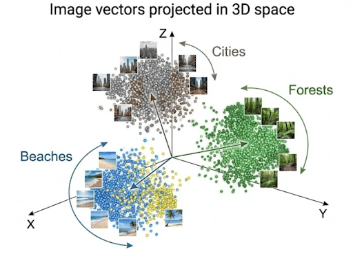
Example 1: Organizing Photographs by Meaning

Imagine you have a collection of vacation photos: beaches, mountains, forests, and cities.

Instead of sorting by file name or date taken, you use a vision model to extract embeddings from each image.

Each photo becomes a vector encoding visual patterns such as:

• dominant colors: blue ocean vs. green forest
• textures: sand vs. snow
• objects: buildings, trees, waves

When you query “mountain scenery”, the system converts your text into a vector and compares it with all stored image vectors.

Those with the closest vectors (i.e., semantically similar content) are retrieved.

This is precisely how Google Photos, Pinterest, and e-commerce visual search systems likely work internally.

---

Example 2: Searching Across Text

Now consider a corpus of thousands of news articles.

A traditional keyword search for “AI regulation in Europe” might miss a document titled “EU passes new AI safety act” because the exact terms differ.

With vector embeddings, both queries and documents live in the same semantic space, so similarity depends on meaning — not exact words.

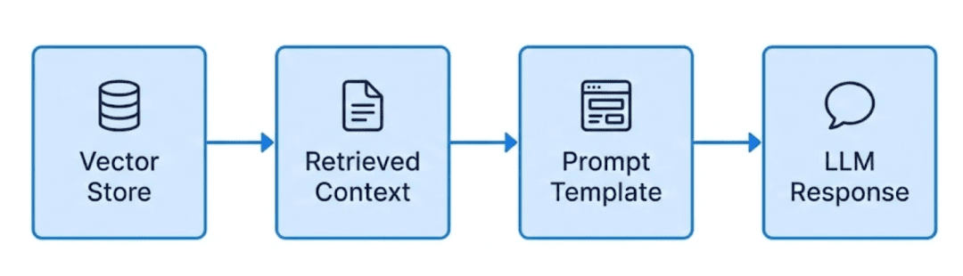
This is the foundation of RAG (Retrieval-Augmented Generation) systems, where retrieved passages (based on embeddings) feed into an LLM to produce grounded answers.

---

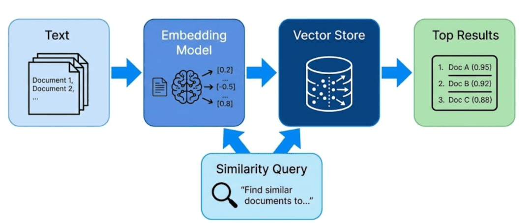
How It Works Conceptually

• Encoding: Convert raw content (text, image, etc.) into dense numerical vectors
• Storing: Save these vectors and their metadata in a vector database
• Querying: Convert an incoming query into a vector and find nearest neighbors
• Returning: Retrieve both the matched embeddings and the original data they represent

This last point is crucial — a vector database doesn’t just store vectors; it keeps both embeddings and raw content aligned.

Otherwise, you’d find “similar” items but have no way to show the user what those items actually were.

Analogy:
Think of embeddings as coordinates, and the vector database as a map that also remembers the real-world landmarks behind each coordinate.

---

Why It’s a Big Deal

Vector databases bridge the gap between raw perception and reasoning.

They allow machines to:

• Understand semantic closeness between ideas
• Generalize beyond exact words or literal matches
• Scale to millions of vectors efficiently using Approximate Nearest Neighbor (ANN) search

You’ll implement that last part — ANN — in Lesson 2, but for now, it’s enough to understand that vector databases make meaning both storable and searchable.

Transition:

Now that you know what vector databases are and why they’re so powerful, let’s look at how we mathematically represent meaning itself — with embeddings.

---

Understanding Embeddings: Turning Language into Geometry

If a vector database is the brain’s memory, embeddings are the neurons that hold meaning.

At a high level, an embedding is just a list of floating-point numbers — but each number encodes a latent feature learned by a model.

Together, these features represent the semantics of an input: what it talks about, what concepts appear, and how those concepts relate.

So when two texts mean the same thing — even if they use different words — their embeddings lie close together in this high-dimensional space.

🧠 Think of embeddings as “meaning coordinates.”
The closer two points are, the more semantically alike their underlying texts are.

---

Why Do We Need Embeddings?

Traditional keyword search works by counting shared words.

But language is flexible — the same idea can be expressed in many forms:

Embeddings fix this by mapping both sentences to nearby vectors — the geometric signal of shared meaning.

---

How Embeddings Work (Conceptually)

When we feed text into an embedding model, it outputs a vector like:

[0.12, -0.45, 0.38, ..., 0.09]

Each dimension encodes latent attributes such as topic, tone, or contextual relationships.

For example:

• “banana” and “apple” might share high weights on a fruit dimension
• “AI model” and “neural network” might align on a technology dimension

When visualized (e.g., with PCA or t-SNE), semantically similar items cluster together — you can literally see meaning from patterns.

---

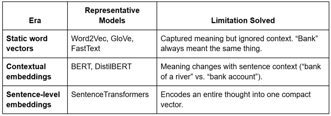
From Static to Contextual to Sentence-Level Embeddings

Embeddings didn’t always understand context.

They evolved through 3 major eras — each addressing a key limitation.

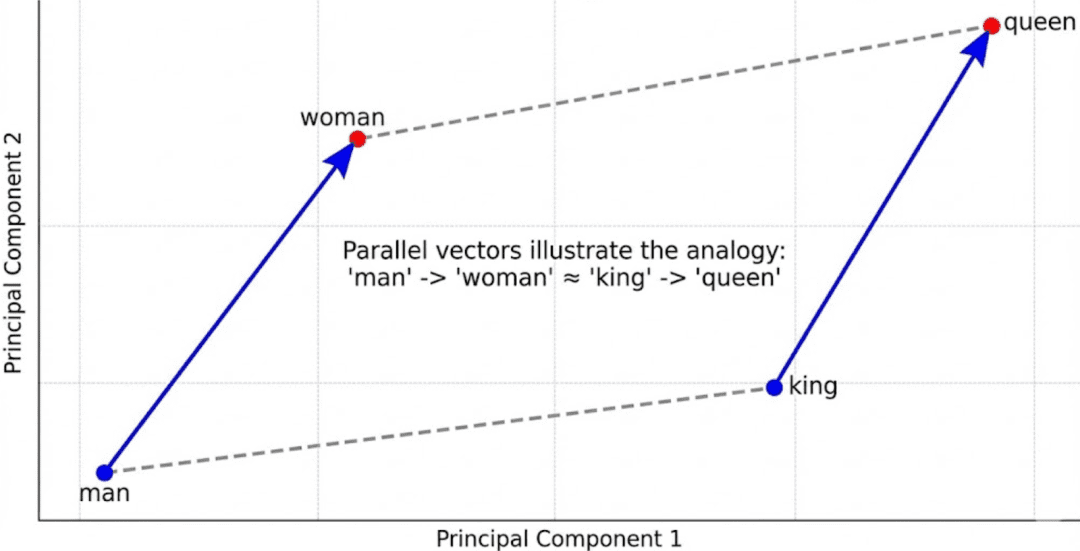
Example: Word2Vec Analogies

Early models such as Word2Vec captured fascinating linear relationships:

King - Man + Woman ≈ Queen
Paris - France + Italy ≈ Rome

These showed that embeddings could represent conceptual arithmetic.

But Word2Vec assigned only one vector per word — so it failed for polysemous words such as table (“spreadsheet” vs. “furniture”).

Callout:
Static embeddings = one vector per word → no context.
Contextual embeddings = different vectors per sentence → true understanding.

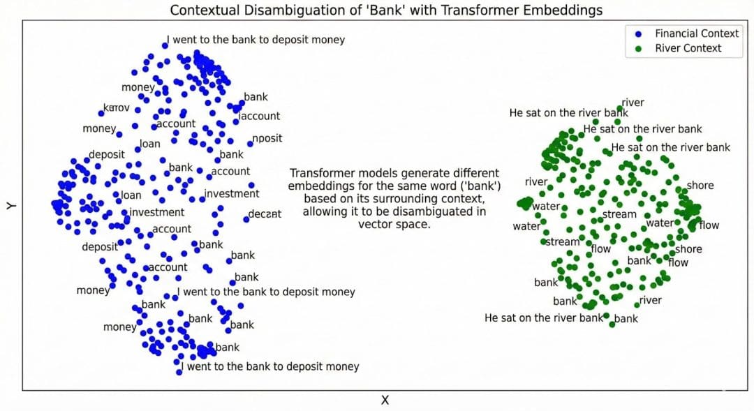
BERT and the Transformer Revolution

Transformers introduced contextualized embeddings via self-attention.

Instead of treating words independently, the model looks at surrounding words to infer meaning.

BERT (Bidirectional Encoder Representations from Transformers) uses 2 training objectives:

• Masked Language Modeling (MLM): randomly hides words and predicts them using context.
• Next Sentence Prediction (NSP): determines whether two sentences follow each other.

This bidirectional understanding made embeddings context-aware — the word “bank” now has distinct vectors depending on usage.

Sentence Transformers

Sentence Transformers (built on BERT and DistilBERT) extend this further — they generate one embedding per sentence or paragraph rather than per word.

That’s exactly what your project uses:
all-MiniLM-L6-v2, a lightweight, high-quality model that outputs 384-dimensional sentence embeddings.

Each embedding captures the holistic intent of a sentence — perfect for semantic search and RAG.

---

How This Maps to Your Code

In pyimagesearch/config.py, you define:

EMBED_MODEL_NAME = "sentence-transformers/all-MiniLM-L6-v2"

That line tells your pipeline which model to load when generating embeddings.

Everything else (batch size, normalization, etc.) is handled by helper functions in pyimagesearch/embeddings_utils.py.

Let’s unpack how that happens.

Loading the Model

from sentence_transformers import SentenceTransformer

def get_model(model_name=config.EMBED_MODEL_NAME):
    return SentenceTransformer(model_name)

This fetches a pretrained SentenceTransformer from Hugging Face, loads it once, and returns a ready-to-use encoder.

Generating Embeddings

def generate_embeddings(texts, model=None, batch_size=16, normalize=True):
    embeddings = model.encode(
        texts, batch_size=batch_size, show_progress_bar=True,
        convert_to_numpy=True, normalize_embeddings=normalize
    )
    return embeddings

Each text line from your corpus (data/input/corpus.txt) is transformed into a 384-dimensional vector.

Normalization ensures all vectors lie on a unit sphere — that’s why later, cosine similarity becomes just a dot product.

Tip: Cosine similarity measures angle, not length.
L2 normalization keeps all embeddings equal-length, so only direction (meaning) matters.

---

Why Embeddings Cluster Semantically

When plotted (using PCA (principal component analysis) or t-SNE (t-distributed stochastic neighbor embedding)), embeddings from similar topics form clusters:

• “vector database,” “semantic search,” “HNSW” (hierarchical navigable small world) → one cluster
• “normalization,” “cosine similarity” → another

That happens because embeddings are trained with contrastive objectives — pushing semantically close examples together and unrelated ones apart.

You’ve now seen what embeddings are, how they evolved, and how your code turns language into geometry — points in a high-dimensional space where meaning lives.

Next, let’s bring it all together.

We’ll walk through the full implementation — from configuration and utilities to the main driver script — to see exactly how this semantic search pipeline works end-to-end.

---

Would you like immediate access to 3,457 images curated and labeled with hand gestures to train, explore, and experiment with … for free? Head over to Roboflow and get a free account to grab these hand gesture images.

---

Configuring Your Development Environment

To follow this guide, you need to install several Python libraries for working with semantic embeddings and text processing.

The core dependencies are:

$ pip install sentence-transformers==2.7.0
$ pip install numpy==1.26.4  
$ pip install rich==13.8.1

---

Verifying Your Installation

You can verify the core libraries are properly installed by running:

from sentence_transformers import SentenceTransformer
import numpy as np
from rich import print

model = SentenceTransformer('all-MiniLM-L6-v2')
print("Environment setup complete!")

Note: The sentence-transformers library will automatically download the embedding model on first use, which may take a few minutes depending on your internet connection.

---

Need Help Configuring Your Development Environment?

All that said, are you:

• Short on time?
• Learning on your employer’s administratively locked system?
• Wanting to skip the hassle of fighting with the command line, package managers, and virtual environments?
• Ready to run the code immediately on your Windows, macOS, or Linux system?

Then join PyImageSearch University today!

Gain access to Jupyter Notebooks for this tutorial and other PyImageSearch guides pre-configured to run on Google Colab’s ecosystem right in your web browser! No installation required.

And best of all, these Jupyter Notebooks will run on Windows, macOS, and Linux!

---

Implementation Walkthrough: Configuration and Directory Setup

Your config.py file acts as the backbone of this entire RAG series.

It defines where data lives, how models are loaded, and how different pipeline components (embeddings, indexes, prompts) talk to each other.

Think of it as your project’s single source of truth — modify paths or models here, and every script downstream stays consistent.

---

Setting Up Core Directories

from pathlib import Path
import os

BASE_DIR = Path(__file__).resolve().parent.parent
DATA_DIR = BASE_DIR / "data"
INPUT_DIR = DATA_DIR / "input"
OUTPUT_DIR = DATA_DIR / "output"
INDEX_DIR = DATA_DIR / "indexes"
FIGURES_DIR = DATA_DIR / "figures"

Each constant defines a key working folder.

• BASE_DIR: dynamically finds the project’s root, no matter where you run the script from
• DATA_DIR: groups all project data under one roof
• INPUT_DIR: your source text (corpus.txt) and optional metadata
• OUTPUT_DIR: cached artifacts such as embeddings and PCA (principal component analysis) projections
• INDEX_DIR: FAISS (Facebook AI Similarity Search) indexes you’ll build in Part 2
• FIGURES_DIR: visualizations such as 2D semantic plots

TIP: Centralizing all paths prevents headaches later when switching between local, Colab, or AWS environments.

---

Corpus Configuration

_CORPUS_OVERRIDE = os.getenv("CORPUS_PATH")
_CORPUS_META_OVERRIDE = os.getenv("CORPUS_META_PATH")
CORPUS_PATH = Path(_CORPUS_OVERRIDE) if _CORPUS_OVERRIDE else INPUT_DIR / "corpus.txt"
CORPUS_META_PATH = Path(_CORPUS_META_OVERRIDE) if _CORPUS_META_OVERRIDE else INPUT_DIR / "corpus_metadata.json"

This lets you override corpus files via environment variables — useful when you want to test different datasets without editing the code.

For instance:

export CORPUS_PATH=/mnt/data/new_corpus.txt

Now, all scripts automatically pick up that new file.

---

Embedding and Model Artifacts

EMBEDDINGS_PATH = OUTPUT_DIR / "embeddings.npy"
METADATA_ALIGNED_PATH = OUTPUT_DIR / "metadata_aligned.json"
DIM_REDUCED_PATH = OUTPUT_DIR / "pca_2d.npy"
FLAT_INDEX_PATH = INDEX_DIR / "faiss_flat.index"
HNSW_INDEX_PATH = INDEX_DIR / "faiss_hnsw.index"
EMBED_MODEL_NAME = "sentence-transformers/all-MiniLM-L6-v2"

Here, we define the semantic artifacts this pipeline will create and reuse.

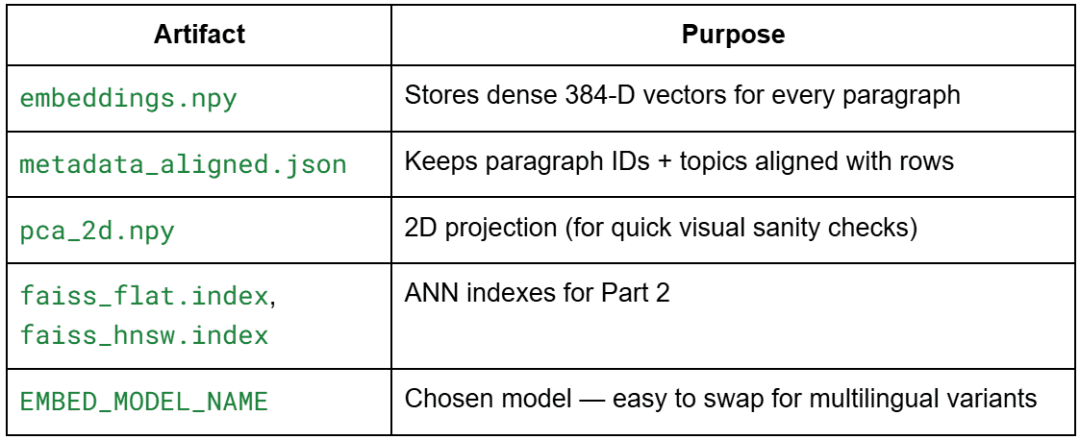
Why all-MiniLM-L6-v2?

It’s lightweight (384 dimensions), fast, and high quality for short passages — perfect for demos.

Later, you can easily replace it with a multilingual or domain-specific model by changing this single variable.

---

General Settings

SEED = 42
DEFAULT_TOP_K = 5
SIM_THRESHOLD = 0.35

These constants control experiment repeatability and ranking logic.

• SEED: keeps PCA and ANN reproducible
• DEFAULT_TOP_K: sets how many neighbors to retrieve for queries
• SIM_THRESHOLD: acts as a loose cutoff to ignore extremely weak matches

---

Optional: Prompt Templates for RAG

Though not yet used in Lesson 1, the config already prepares the RAG foundation:

STRICT_SYSTEM_PROMPT = (
    "You are a concise assistant. Use ONLY the provided context."
    " If the answer is not contained verbatim or explicitly, say you do not know."
)
SYNTHESIZING_SYSTEM_PROMPT = (
    "You are a concise assistant. Rely ONLY on the provided context, but you MAY synthesize"
    " an answer by combining or paraphrasing the facts present."
)
USER_QUESTION_TEMPLATE = "User Question: {question}nAnswer:"
CONTEXT_HEADER = "Context:"

This anticipates how the retriever (vector database) will later feed context chunks into a language model.

In Part 3, you’ll use these templates to construct dynamic prompts for your RAG pipeline.

---

Final Touch

for d in (OUTPUT_DIR, INDEX_DIR, FIGURES_DIR):
    d.mkdir(parents=True, exist_ok=True)

A small but powerful line — ensures all directories exist before writing any files.

You’ll never again get the “No such file or directory” error during your first run.

In summary, config.py defines the project’s constants, artifacts, and model parameters — keeping everything centralized, reproducible, and RAG-ready.

Next, we’ll move to embeddings_utils.py, where you’ll load the corpus, generate embeddings, normalize them, and persist the artifacts.

---

Embedding Utilities (embeddings_utils.py)

---

Overview

This module powers everything you’ll do in Lesson 1. It provides reusable, modular functions for:

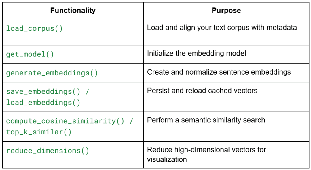
Each function is deliberately stateless — you can plug them into other projects later without modification.

---

Loading the Corpus

def load_corpus(corpus_path=CORPUS_PATH, meta_path=CORPUS_META_PATH):
    with open(corpus_path, "r", encoding="utf-8") as f:
        texts = [line.strip() for line in f if line.strip()]
    if meta_path.exists():
        import json; metadata = json.load(open(meta_path, "r", encoding="utf-8"))
    else:
        metadata = []
    if len(metadata) != len(texts):
        metadata = [{"id": f"p{idx:02d}", "topic": "unknown", "tokens_est": len(t.split())} for idx, t in enumerate(texts)]
    return texts, metadata

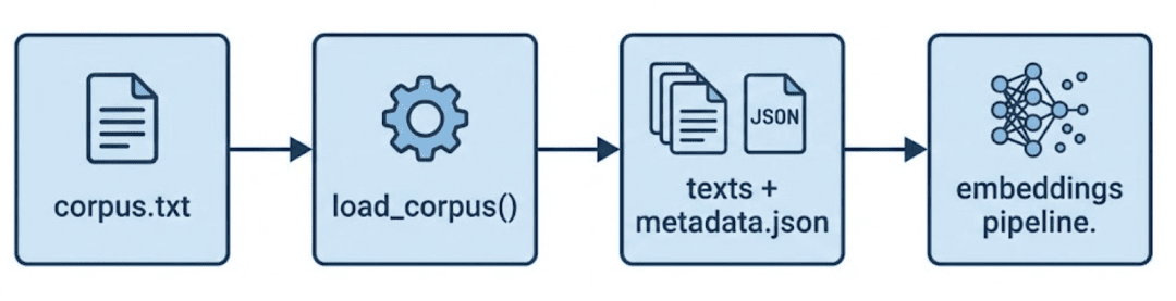
This is the starting point of your data flow.

It reads each non-empty paragraph from your corpus (data/input/corpus.txt) and pairs it with metadata entries.

Why It Matters

• Guarantees alignment — each embedding always maps to its original text
• Automatically repairs metadata if mismatched or missing
• Prevents silent data drift during re-runs

TIP: In later lessons, this alignment ensures the top-k search results can be traced back to their paragraph IDs or topics.

---

Loading the Embedding Model

from sentence_transformers import SentenceTransformer

def get_model(model_name=EMBED_MODEL_NAME):
    return SentenceTransformer(model_name)

This function centralizes model loading.

Instead of hard-coding the model everywhere, you call get_model() once — making the rest of your pipeline model-agnostic.

Why This Pattern

• Let’s you swap models easily (e.g., multilingual or domain-specific)
• Keeps the driver script clean
• Prevents re-initializing the model repeatedly (you’ll reuse the same instance)

Model insight:
all-MiniLM-L6-v2 has 22 M parameters and produces 384-dimensional embeddings.

It’s fast enough for local demos yet semantically rich enough for clustering and similarity ranking.

---

Generating Embeddings

import numpy as np

def generate_embeddings(texts, model=None, batch_size: int = 16, normalize: bool = True):
    if model is None: model = get_model()
    embeddings = model.encode(
        texts,
        batch_size=batch_size,
        show_progress_bar=True,
        convert_to_numpy=True,
        normalize_embeddings=normalize
    )
    if normalize:
        norms = np.linalg.norm(embeddings, axis=1, keepdims=True)
        norms[norms == 0] = 1.0
        embeddings = embeddings / norms
    return embeddings

This is the heart of Lesson 1 — converting human language into geometry.

What Happens Step by Step

1. Encode text: Each sentence becomes a dense vector of 384 floats
2. Normalize: Divides each vector by its L2 norm so it lies on a unit hypersphere
3. Return NumPy array: Shape → (n_paragraphs × 384)

Why Normalization?

Because cosine similarity depends on vector direction, not length.

L2 normalization makes cosine = dot product — faster and simpler for ranking.

Mental model:
Each paragraph now “lives” somewhere on the surface of a sphere where nearby points share similar meaning.

---

Saving and Loading Embeddings

import json

def save_embeddings(embeddings, metadata, emb_path=EMBEDDINGS_PATH, meta_out_path=METADATA_ALIGNED_PATH):
    np.save(emb_path, embeddings)
    json.dump(metadata, open(meta_out_path, "w", encoding="utf-8"), indent=2)

def load_embeddings(emb_path=EMBEDDINGS_PATH, meta_out_path=METADATA_ALIGNED_PATH):
    emb = np.load(emb_path)
    meta = json.load(open(meta_out_path, "r", encoding="utf-8"))
    return emb, meta

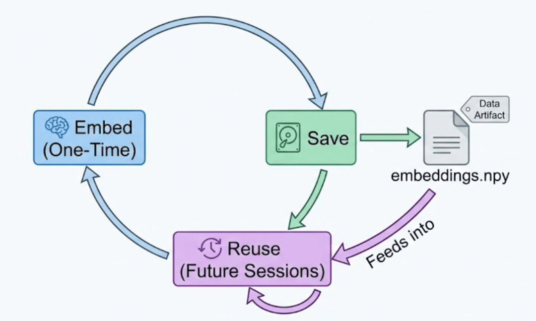
Caching is essential once you have expensive embeddings. These two helpers store and reload them in seconds.

Why Both .npy and .json?

• .npy: fast binary format for numeric data
• .json: human-readable mapping of metadata to embeddings

Good practice:
Never modify metadata_aligned.json manually — it ensures row consistency between text and embeddings.

---

Computing Similarity and Ranking

def compute_cosine_similarity(vec, matrix):
    return matrix @ vec

def top_k_similar(query_emb, emb_matrix, k=DEFAULT_TOP_K):
    sims = compute_cosine_similarity(query_emb, emb_matrix)
    idx = np.argpartition(-sims, k)[:k]
    idx = idx[np.argsort(-sims[idx])]
    return idx, sims[idx]

These two functions transform your embeddings into a semantic search engine.

How It Works

• compute_cosine_similarity: performs a fast dot-product of a query vector against the embedding matrix
• top_k_similar: picks the top-k results without sorting all N entries — efficient even for large corpora

Analogy:
Think of it like Google search, but instead of matching words, it measures meaning overlap via vector angles.

Complexity:
O(N × D) per query — acceptable for small datasets, but this sets up the motivation for ANN indexing in Lesson 2.

---

Reducing Dimensions for Visualization

from sklearn.decomposition import PCA

def reduce_dimensions(embeddings, n_components=2, seed=42):
    pca = PCA(n_components=n_components, random_state=seed)
    return pca.fit_transform(embeddings)

Why PCA?

• Humans can’t visualize 384-D space
• PCA compresses to 2-D while preserving the largest variance directions
• Perfect for sanity-checking that semantic clusters look reasonable

Remember: You’ll still perform searches in 384-D — PCA is for visualization only.

At this point, you have:

• Clean corpus + metadata alignment
• A working embedding generator
• Normalized vectors ready for cosine similarity
• Optional visualization via PCA

All that remains is to connect these utilities in your main driver script (01_intro_to_embeddings.py), where we’ll orchestrate embedding creation, semantic search, and visualization.

---

Driver Script Walkthrough (01_intro_to_embeddings.py)

The driver script doesn’t introduce new algorithms — it wires together all the modular utilities you just built.

Let’s go through it piece by piece so you understand not only what happens but why each part belongs where it does.

---

Imports and Setup

import numpy as np
from rich import print
from rich.table import Table

from pyimagesearch import config
from pyimagesearch.embeddings_utils import (
    load_corpus,
    generate_embeddings,
    save_embeddings,
    load_embeddings,
    get_model,
    top_k_similar,
    reduce_dimensions,
)

Explanation

• You’re importing helper functions from embeddings_utils.py and configuration constants from config.py.
• rich is used for pretty-printing output tables in the terminal — adds color and formatting for readability.
• Everything else (numpy, reduce_dimensions, etc.) was already covered; we’re just combining them here.

---

Ensuring Embeddings Exist or Rebuilding Them

def ensure_embeddings(force: bool = False):
    if config.EMBEDDINGS_PATH.exists() and not force:
        emb, meta = load_embeddings()
        texts, _ = load_corpus()
        return emb, meta, texts
    texts, meta = load_corpus()
    model = get_model()
    emb = generate_embeddings(texts, model=model, batch_size=16, normalize=True)
    save_embeddings(emb, meta)
    return emb, meta, texts

What This Function Does

This is your entry checkpoint — it ensures you always have embeddings before doing anything else.

• If cached .npy and .json files exist → simply load them (no recomputation)
• Otherwise → read the corpus, generate embeddings, save them, and return

Why It Matters

• Saves you from recomputing embeddings every run (a huge time saver)
• Keeps consistent mapping between text ↔ embedding across sessions
• The force flag lets you rebuild from scratch if you change models or data

TIP: In production, you’d make this a CLI (command line interface) flag like --rebuild so that automation scripts can trigger a full re-embedding if needed.

---

Showing Nearest Neighbors (Semantic Search Demo)

def show_neighbors(embeddings: np.ndarray, texts, model, queries):
    print("[bold cyan]nSemantic Similarity Examples[/bold cyan]")
    for q in queries:
        q_emb = model.encode([q], convert_to_numpy=True, normalize_embeddings=True)[0]
        idx, scores = top_k_similar(q_emb, embeddings, k=5)
        table = Table(title=f"Query: {q}")
        table.add_column("Rank")
        table.add_column("Score", justify="right")
        table.add_column("Text (truncated)")
        for rank, (i, s) in enumerate(zip(idx, scores), start=1):
            snippet = texts[i][:100] + ("..." if len(texts[i]) > 100 else "")
            table.add_row(str(rank), f"{s:.3f}", snippet)
        print(table)

Step-by-Step

• Loop over each natural-language query (e.g., “Explain vector databases”)
• Encode it into a vector via the same model — ensuring semantic consistency
• Retrieve top-k similar paragraphs via cosine similarity.
• Render the result as a formatted table with rank, score, and a short snippet

What This Demonstrates

• It’s your first real semantic search — no indexing yet, but full meaning-based retrieval
• Shows how “nearest neighbors” are determined by semantic closeness, not word overlap
• Sets the stage for ANN acceleration in Lesson 2

OBSERVATION: Even with only 41 paragraphs, the search feels “intelligent” because the embeddings capture concept-level similarity.

---

Visualizing the Embedding Space

def visualize(embeddings: np.ndarray):
    coords = reduce_dimensions(embeddings, n_components=2)
    np.save(config.DIM_REDUCED_PATH, coords)
    try:
        import matplotlib.pyplot as plt
        fig_path = config.FIGURES_DIR / "semantic_space.png"
        plt.figure(figsize=(6, 5))
        plt.scatter(coords[:, 0], coords[:, 1], s=20, alpha=0.75)
        plt.title("PCA Projection of Corpus Embeddings")
        plt.tight_layout()
        plt.savefig(fig_path, dpi=150)
        print(f"Saved 2D projection to {fig_path}")
    except Exception as e:
        print(f"[yellow]Could not generate plot: {e}[/yellow]")

Why Visualize?

Visualization makes abstract geometry tangible.

PCA compresses 384 dimensions into 2, so you can see whether related paragraphs are clustering together.

Implementation Notes

• Stores projected coordinates (pca_2d.npy) for re-use in Lesson 2.
• Gracefully handles environments without display backends (e.g., remote SSH (Secure Shell)).
• Transparency (alpha=0.75) helps overlapping clusters remain readable.

---

Main Orchestration Logic

def main():
    print("[bold magenta]Loading / Generating Embeddings...[/bold magenta]")
    embeddings, metadata, texts = ensure_embeddings()
    print(f"Loaded {len(texts)} paragraphs. Embedding shape: {embeddings.shape}")

    model = get_model()

    sample_queries = [
        "Why do we normalize embeddings?",
        "What is HNSW?",
        "Explain vector databases",
    ]
    show_neighbors(embeddings, texts, model, sample_queries)

    print("[bold magenta]nCreating 2D visualization (PCA)...[/bold magenta]")
    visualize(embeddings)

    print("[green]nDone. Proceed to Post 2 for ANN indexes.n[/green]")


if __name__ == "__main__":
    main()

Flow Explained

• Start → load or build embeddings
• Run semantic queries and show top results
• Visualize 2D projection
• Save everything for the next lesson

The print colors (magenta, cyan, green) help readers follow the stage progression clearly when running in the terminal.

---

Example Output (Expected Terminal Run)

When you run:

python 01_intro_to_embeddings.py

You should see something like this in your terminal:

---

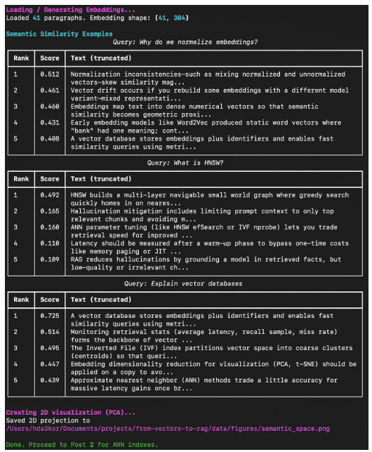
What You’ve Built So Far

• A mini semantic search engine that retrieves paragraphs by meaning, not keyword
• Persistent artifacts (embeddings.npy, metadata_aligned.json, pca_2d.npy)
• Visualization of concept clusters that proves embeddings capture semantics

This closes the loop for Lesson 1: Understanding Vector Databases and Embeddings — you’ve implemented everything up to the baseline semantic search.

---

---

Summary

In this lesson, you built the foundation for understanding how machines represent meaning.

You began by revisiting the limitations of keyword-based search — where two sentences can express the same intent yet remain invisible to one another because they share few common words. From there, you explored how embeddings solve this problem by mapping language into a continuous vector space where proximity reflects semantic similarity rather than mere token overlap.

You then learned how modern embedding models (e.g., SentenceTransformers) generate these dense numerical vectors. Using the all-MiniLM-L6-v2 model, you transformed every paragraph in your handcrafted corpus into a 384-dimensional vector — a compact representation of its meaning. Normalization ensured that every vector lay on the unit sphere, making cosine similarity equivalent to a dot product.

With those embeddings in hand, you performed your first semantic similarity search. Instead of counting shared words, you compared the direction of meaning between sentences and observed how conceptually related passages naturally rose to the top of your rankings. This hands-on demonstration illustrated the power of geometric search — the bridge from raw language to understanding.

Finally, you visualized this semantic landscape using PCA, compressing hundreds of dimensions down to two. The resulting scatter plot revealed emergent clusters: paragraphs about normalization, approximate nearest neighbors, and vector databases formed their own neighborhoods. It’s a visual confirmation that the model has captured genuine structure in meaning.

By the end of this lesson, you didn’t just learn what embeddings are — you saw them in action. You built a small but complete semantic engine: loading data, encoding text, searching by meaning, and visualizing relationships. These artifacts now serve as the input for the next stage of the journey, where you’ll make search truly scalable by building efficient Approximate Nearest Neighbor (ANN) indexes with FAISS.

In Lesson 2, you’ll learn how to speed up similarity search from thousands of comparisons to milliseconds — the key step that turns your semantic space into a production-ready vector database.

---

Citation Information

Singh, V. “TF-IDF vs. Embeddings: From Keywords to Semantic Search,” PyImageSearch, P. Chugh, S. Huot, A. Sharma, and P. Thakur, eds., 2026, https://pyimg.co/msp43

@incollection{Singh_2026_tf-idf-vs-embeddings-from-keywords-to-semantic-search,
  author = {Vikram Singh},
  title = {{TF-IDF vs. Embeddings: From Keywords to Semantic Search}},
  booktitle = {PyImageSearch},
  editor = {Puneet Chugh and Susan Huot and Aditya Sharma and Piyush Thakur},
  year = {2026},
  url = {https://pyimg.co/msp43},
}

---

To download the source code to this post (and be notified when future tutorials are published here on PyImageSearch), simply enter your email address in the form below!

The post TF-IDF vs. Embeddings: From Keywords to Semantic Search appeared first on PyImageSearch.