RAG — Full Matrix Evaluation

digitado ⋅ 7 de February de 2026

RAG — Retrieval Full Matrix Evaluation

1 ] Introduction

Choosing the right retrieval model is often the “make or break” moment for any Retrieval-Augmented Generation (RAG) system. While many developers focus on the LLM, the quality of the response is strictly limited by the quality of the retrieved data. Previously, I wrote about the common mistakes engineers make when developing RAG systems and the hallucinations they can generate. This article takes a step back to the preliminary phase of analysis and prototyping that should occur before any project deployment.

While developing a RAG system for a client, I prepared this ready-to-use evaluation matrix to help you (and me) navigating the evaluation of the many components that make up a retrieval system.

Throughout this article, I have used a 3-point scoring system for my evaluation tables. While the specific thresholds for each score are relative to the specific use case, I find this system incredibly valuable for communication. It allows me to translate complex technical findings into a clear, accessible format for non-technical colleagues and stakeholders.

1.1 ] System Architecture Based on Vector Datasets

It is always a challenge to know exactly who will be reading my articles and how much experience they have with RAG. To make sure no one gets lost, I’ll spend a few more paragraphs explaining the two steps of the retrieval process. This context is vital for making sense of the evaluation metrics we are about to cover.

A retrieval system is designed to operate on two logically and temporally separate levels.

Phase 1 — Indexing (Offline/Batch):

Document Upload → Content Extraction → Chunking → Embedding Calculation (ONCE) → Storage (ES/OpenSearch)

In this initial phase, which occurs in batch or offline mode, the system handles document “ingestion.” When a file is uploaded, the content is extracted, divided into small fragments (chunks), and transformed into numerical vectors through embedding calculation.

It is important to note that this operation is performed only once per document: once generated, the embeddings are permanently saved in the database (e.g. ES/OpenSearch). Since this is a background process, it is not a critical phase regarding user wait times. This allows us to optimize the system for handling large volumes of data (throughput) and to utilize parallelization.

Phase 2 — Search (Online/Real-time):

User Query → Query Embedding Calculation → Similarity Search in ES/OpenSearch → Result Ranking → Response

When a user submits a question, the system must instantaneously calculate the embedding for that query and compare it with those stored in the database to find the most relevant results.

In this phase, latency is the crucial factor: the user is waiting, and every millisecond counts for a smooth experience.

Strategic Implications This clear separation radically changes how we must evaluate system success. Performance criteria follow two distinct tracks:

Top Priority for Search: Evaluation must focus on query latency and response speed (QPS). This is where the user’s perception of quality is determined.
Secondary Priority for Indexing: Here, the key parameters are throughput (documents processed per minute) and the efficiency of batch processes. A slight delay in this phase is acceptable, as it does not interrupt the end-user’s workflow.

2 ] Evaluation Criteria

2.1 ] Embedder Characteristics

Requirement: The physical architecture of the model determines the system’s operational costs and scalability.

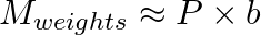
Memory Footprint. The static memory occupied by the model parameters when loaded depends on the number of parameters (P) (e.g., 100M, 500M, 1B) and the data precision (number of bytes per parameter b).

FP32 (Single Precision): b = 4 bytes
FP16/BF16 (Half Precision): b = 2 bytes
INT8 (Quantized): b = 1 byte

Uniform Encoding and Shared Space. At times, multilingual capability is a structural requirement. A multilingual model produces a shared vector space, ensuring, for example, that the concept of “mela” (IT) and “apple” (EN) occupy the same numerical coordinates. Without this feature, it would be necessary to translate every query before searching, increasing system complexity while losing time and precision.

2.2 ] Semantic Search Quality

Requirement: The Retrieval Quality requirement defines the model’s effectiveness in identifying and retrieving documents from the vector store that contain the answer or the information semantically necessary to satisfy the user’s query.

There are many metrics we could talk about but the performance is typically expressed as Recall@K, which measures the system’s ability to find all relevant documents present in the database within the top K results returned (usually K=10 or K=50). Put simply: “Out of K searches performed, how many times did the model place the most relevant documents in the very top positions of the ranking?”

If we know that 10 relevant documents exist in the system for a specific query and the model finds 8 of them within the top 10 results, the Recall@10 will be 80%.

Note: Quality thresholds must always be interpreted in relation to:

The value of K used (e.g., Recall@5, Recall@10, Recall@50).
The total number of relevant documents for the query in the evaluation dataset.

Higher recall values are generally harder to achieve when the number of relevant documents increases or when K is very low. It also depends on the difficulty of the task itself. Therefore, we refer to the measures cited above, though they may be slightly adapted to specific scenarios.

Hybrid-search (semantic + metadata): The system combines vector similarity with structured filters (e.g., category, date, language, tags). It measures the ability to retrieve semantically correct documents while respecting filter constraints.
Monolingual Retrieval: Query and documents are in the same language. This evaluates the pure accuracy of the semantic engine without complexities arising from translation or cross-lingual alignment.
Cross-lingual Retrieval: Query and documents are in different languages (e.g., query in Italian, documents in English). It measures the model’s ability to represent multilingual content in the same vector space and retrieve relevant documents without explicit translation.

2.3 ] Latency & Query Throughput

In Retrieval architectures, real-time performance is defined by the dynamic balance between Latency and Throughput.

2.3.1 ] Latency

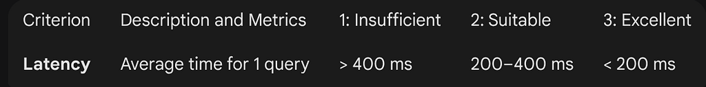
Requirement: Latency is the time interval between the moment an input is sent (the user query) and the moment the output becomes available (the display of results).

The latency formula can be expressed as:

Each term in the formula represents a specific optimization point:

ΔTₑ (Inference Delta): The time required to transform the text query into a numerical vector via the embedding model.
ΔTₛ (Vector Search Delta): The time taken by the database (Elasticsearch/OpenSearch) to navigate the index (e.g., HNSW) and find the k nearest neighbors.
ΔTᵣ (Post-processing Delta): Time dedicated to any potential re-ordering of results (Reranking) or applying scalar filters (e.g., filters by date or user permissions). Optional depending on the final archirecture.

These KPIs refer to [1]

2.3.2 ] Query Throughput

Requirement: Throughput (TH) represents the production capacity of the system, i.e., the volume of search requests the infrastructure can successfully process per unit of time (typically expressed in Queries Per Second, QPS).

The general formula can be expressed as:

Where:

N: Number of requests processed in parallel.
ΔL: Average total latency per query.

Throughput is influenced by three critical bottlenecks that must be balanced to avoid performance degradation:

Computational Saturation (ΔTₑ + ΔTᵣ): Embedding calculation is an intensive operation. If the number of parallel requests exceeds the hardware’s simultaneous computing capacity, queries begin to form wait queues, artificially increasing perceived latency.
Search Engine Efficiency (ΔTₛ): The speed at which the vector database navigates the HNSW index. High throughput requires the index structure to be readily accessible (preferably in RAM) to minimize I/O wait times.
Concurrency Management: The architecture must correctly handle resource locking and load distribution across cluster nodes (Load Balancing).

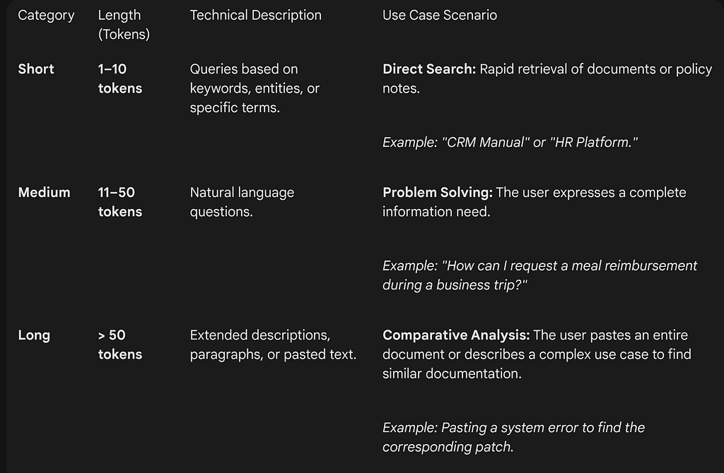
2.3.3 ] Query Categorization

Both ΔL and TH depend directly on the length of the customer queries. To correctly define performance benchmarks, it is useful to categorize queries based on the number of tokens, as the computational effort required from the embedding model — and thus the response times — depends on this. The below table represents an attempt to find this characterization. However, other taxonomies might be more relative depending on the specific case.

Below, I also describe plausible tests for the two previous metrics, incorporating everything discussed so far.

2.3.4 ] Load Simulation

The objective of this test is to map the system’s behavior under stress, identifying the direct link between request volume (Input QPS), processing capacity (Throughput), and user experience quality (Latency).

Input Variables:

Database Size: Total number of indexed documents in the vector store.
Model Size: Number of parameters in the chosen embedding architecture.
Vector Dimensions: Dimensionality of the vector space (e.g., 768 or 1536).
Input Rate (Sent QPS): The controlled stress level expressed in Queries Per Second.

Output Variables:

Throughput (Effective QPS): The number of requests the system successfully completes per unit of time.
Latency (Response Time): The end-to-end time measured at P50 (median) and P95 (stability) percentiles. This includes computation time and any potential queueing delay.

In the Isolated Characterization Test, the system is tested by sending homogeneous loads per category. This serves to isolate the computational cost of encoding (ΔTₑ) based on text length.

To simulate a real production environment, a Mixed Stress Test might also be performed with a weighted distribution. This test is the most representative for defining final hardware sizing.

Load Distribution:

60% Short Queries (Quick search)
35% Medium Queries (Natural language questions)
5% Long Queries (Document/log analysis)

Testing Method

The following protocol must be executed at different population stages of the Vector Store (e.g., 100k, 1M, 10M documents), model sizes, and vector dimensions to map the scalability curve.

Scalar Stress Analysis: Measure performance metrics by setting an increasing Input Rate at 10, 100, and 1000 QPS. Queries should be extracted both in isolation and using the defined mixed distribution.
Latency Percentile Detection: For each load step, calculate the Mean, P50 (median), P95, and P99. Focus must be placed on high percentiles (P95/P99) to identify queueing delay phenomena.
Hardware Benchmarking: Run the same tests comparatively on CPU and GPU (if available) to quantify the throughput gain provided by hardware acceleration during the ΔTₑ phase.
Saturation Point Identification: Identify the maximum QPS value within which the system maintains a P95 latency < 200ms. Exceeding this threshold identifies the operational limit of the infrastructure.
Sustained Load Test: Maintain a constant traffic rate equal to 80% of the identified maximum QPS for a duration of 1 hour.
Maximum System Capacity: Verify the maximum number of queries the system can handle without encountering an OOM (Out of Memory) error.

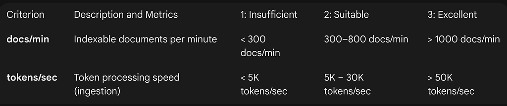
2.4 ] Indexing Throughput

Requirement: Indexing Throughput measures the efficiency with which the system “ingests” new data. It represents the speed of transforming raw documents into stored vectors ready for search.

The primary metrics used are the number of documents or tokens processed per unit of time:

Docs/min (Documents per minute): Useful for a macroscopic view of the load.
Tokens/sec (Tokens per second): The most precise metric, as it normalizes the variable length of documents and reflects the actual computational effort of the embedding model.

Indexing efficiency can be expressed as:

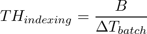
Where:

B: Batch Size (number of documents per call).
ΔT: Batch processing time (including Chunking, Embedding, and disk writing).

Testing Method

Dataset Preparation: Generate a controlled test set of 1,000 documents with a representative length distribution (range of 100–500 tokens).
Batch Size Optimization: Run indexing cycles testing increasing batches: 16, 32, 64, 128, 256. The goal is to identify the trade-off where memory usage (VRAM/RAM) is maximized but stable, avoiding OOM (Out Of Memory) errors.
Hardware Benchmarking: Perform the same tests comparatively on CPU and GPU (if available) to quantify the throughput gain.

2.5 ] Hardware Requirements & Computational Efficiency

Requirement: The choice of the embedding model and search infrastructure is strictly constrained by available hardware resources. The objective is to maximize the ratio between performance (QPS) and operational costs.

Resource allocation depends on three critical factors of the chosen model:

Model Size (Parameters): Directly influences memory consumption and calculation times.
Vector Dimensionality (d): Larger vectors linearly increase RAM occupancy in the Vector Store and slow down cosine similarity calculations.
Numerical Precision (Quantization): Using Float32 weights requires double the memory compared to Float16 or BFloat16. Quantization techniques (INT8/Binary) can drastically reduce hardware impact with minimal loss of precision.

Inference Memory. This is the RAM (or VRAM, in the case of a GPU) dedicated exclusively to the embedding model. It does not depend on the number of documents in the database but rather on the complexity of the model itself.

Static Footprint: The space occupied by the model weights immediately upon loading.
Dynamic Overhead: During query calculation, memory fluctuates based on sequence length (number of tokens) and batch size. If the system must process many simultaneous queries, this overhead can become significant and cause bottlenecks if not correctly dimensioned.

Unlike previous metrics, I don’t find it useful to give absolute scoring points. Hardware needs are intrinsically tied to your specific latency and throughput targets. Instead of seeking a fixed score, the goal should be to identify the minimum memory overhead required to sustain your desired performance levels — nothing more, nothing less.

2.6 ] Estimated Index Size

Requirement: The space required to store document representations directly influences storage costs and search speed across large data volumes.

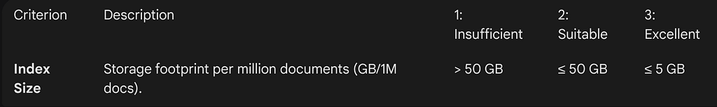
According to the analysis in [2], the impact on storage varies drastically based on the architecture:

Dense Models (Bi-Encoders): These represent each document with a single vector (k=1). They are the most efficient for scalability (e.g., ~2.6 GB per 1M documents with D=768).
Late-Interaction Models (e.g., ColBERT): These store a vector for every token in the document (k = document length). While this approach offers extremely high precision, it requires a memory footprint up to 100 times larger than dense models (e.g., ~900 GB for 15M documents).

2.7 ] Licensing and Deployment Constraints

Here is a point often overlooked: to ensure maximum operational freedom and full legal compliance, my selection of models is strictly limited to those with permissive open-source licenses (such as Apache 2.0 or MIT). Keep in mind that not all dense embedding models are published under these licenses; many are restricted to non-commercial use.

3 ] Conclusion

At the end of this long list I would like to pass a simple message: the “perfect” model doesn’t exist in a vacuum; the best model is the one that fits within your hardware constraints while meeting your users’ latency expectations and your stakeholders’ legal requirements.

By using this evaluation matrix, the selection process moves from a series of “gut feelings” into a data-driven engineering decision.

RAG — Full Matrix Evaluation was originally published in Towards AI on Medium, where people are continuing the conversation by highlighting and responding to this story.

Like 0

Liked Liked