")
Word Embeddings in NLP: From Bag-of-Words to Transformers (Part 1)

· 1. Introduction: Why Computers Struggle with Language
· 2. What Are Word Embeddings and Why Do We Need Them?
∘ The Map Analogy
∘ Why We Need Them
∘ Word embeddings fix this by encoding meaning:
∘ The Core Idea
∘ Why This Revolutionized NLP
· 3. Types of Word Embeddings: From Simple to Sophisticated
∘ The Three Generations
∘ Why This Progression Matters
· 3.1 Frequency-Based Embeddings (The Starting Point)
∘ 3.1.1. Bag-of-Words (BoW)
∘ 3.1.2. TF-IDF (Term Frequency-Inverse Document Frequency)
∘ 3.1.3. N-grams
· 4. Choosing Between Frequency-Based Methods: Quick Guide
∘ The Decision Tree
∘ Quick Comparison Table
∘ Decision Guide by Task Type
∘ Common Mistakes to Avoid
∘ Quick Checklist: Have You Chosen Right?
· 5. Final Thoughts
∘ What I’ve Learned
∘ What’s Next
· 6. Resources & Further Learning
1. Introduction: Why Computers Struggle with Language
I’ll never forget my first attempt at building a sentiment analysis model. I had a dataset of product reviews, some Python knowledge, and a lot of confidence. The plan seemed simple: count the words, feed them to a model, and boom — instant sentiment classifier.
It failed miserably.
The model couldn’t understand the relationships between words. It had no idea that “awful” and “terrible” express similar negativity, or that “awesome” and “excellent” both mean strong positivity. To the model, every word was just an isolated feature with no connection to any other word. And when someone wrote “This product isn’t bad,” the model saw “bad” and classified it as negative, ignoring the “isn’t.”
That’s when I realised: computers don’t understand language the way we do.
We humans, get meaning instantly. We know “king” relates to “queen,” that “huge” and “gigantic” mean similar things, and that “bank” means something different in “river bank” versus “bank account.” We understand context, nuance, and relationships between words.
But computers? They only understand numbers. And the obvious way to convert words to numbers — just assigning each word a unique number — doesn’t capture any of this meaning. To a computer, “cat” as number 5 and “dog” as number 10 have no relationship, even though we know they’re both animals, both pets, both commonly discussed together.
This is the fundamental problem that word embeddings solve: they turn words into numbers in a way that preserves meaning and relationships.
During my Gen AI course, learning about word embeddings was one of those “everything clicks” moments. Suddenly, I understood why my early NLP attempts failed and how modern systems like ChatGPT can actually understand language. Word embeddings bridge the gap between how computers process information (numbers) and how language actually works (meaning and relationships).
In this article, I’ll walk you through:
- What word embeddings actually are and why they’re crucial
- The evolution from simple frequency-based methods to sophisticated contextual embeddings
- Every major type of embedding: when to use it, its strengths, and its limitations
- How to choose the right embedding for your specific task
- Common mistakes I’ve seen (and made) and how to avoid them
Whether you’re building your first NLP model or just trying to understand how modern AI handles language, this guide will give you the foundation you need.
Let’s start with the basics.
2. What Are Word Embeddings and Why Do We Need Them?
Here’s the simplest way I can explain word embeddings: they represent words as points in a multi-dimensional space, where the distance and direction between points capture meaning.
That probably sounds abstract, so let me use an analogy.
The Map Analogy
Think about a map of your city. Every location has coordinates — two numbers that tell you exactly where it is. For example:
Coffee Shop: (40.7580, -73.9855)
Bakery next door: (40.7582, -73.9853)
Your home: (44.7128, -77.0060)
Here’s the interesting part: the distance between coordinates tells you something meaningful. The coffee shop at (40.7580, -73.9855) and the bakery at (40.7582, -73.9853) have very similar coordinates because they’re actually next to each other. Your home at (44.7128, -77.0060) has quite different coordinates because it’s miles away.
The coordinates themselves might look like random numbers, but the relationships between them capture real‑world proximity.
Word embeddings work the same way, but instead of mapping physical locations, we’re mapping words in a “meaning space”. Words with similar meanings end up close to each other. Words that appear in similar contexts are nearby. And the direction between words can even capture relationships.
Here’s a real example that blew my mind when I first saw it:
vector("king") - vector("man") + vector("woman") ≈ vector("queen")
The mathematical relationship between these word vectors actually captures the conceptual relationship between the words. The difference between “king” and “man” is similar to the difference between “queen” and “woman” — both represent a gender relationship in royalty.
Why We Need Them
Let’s go back to my sentiment analysis failure. When I first tried it, I was essentially doing this:
"good" → 1
"bad" → 2
"awesome" → 3
"terrible" → 4
Just random numbers. The computer had no idea that “good” and “awesome” are similar, or that “bad” and “terrible” are similar. Every word was equally different from every other word.
Word embeddings fix this by encoding meaning:
"good" → [0.2, 0.8, 0.1, ...]
"awesome" → [0.3, 0.9, 0.1, ...]
"bad" → [-0.2, -0.7, 0.1, ...]
"terrible" → [-0.3, -0.8, 0.0, ...]
These aren’t random numbers — each dimension captures some aspect of meaning. Now, when the computer processes these vectors, it can see that “good” and “awesome” are similar (their vectors are close), and both are opposite to “bad” and “terrible” (notice the negative values).
The Core Idea
Word embeddings capture three crucial things:
- Semantic Similarity
Words with similar meanings have similar embeddings. “huge,” “gigantic,” and “enormous” all cluster together in the embedding space. - Contextual Relationships
Words that appear in similar contexts are represented similarly. If “coffee” and “tea” often appear in similar sentences (“I’ll have a ___”), their embeddings will be close. - Analogical Reasoning
The relationships between words are captured in the geometry of the space. Not just king→queen, but also:
- Paris→France ≈ London→England (capital-country relationships)
- Walking→Walked ≈ Swimming→Swam (verb tense relationships)
- Fast→Faster ≈ Strong→Stronger (comparative relationships)
Why This Revolutionised NLP
Before word embeddings, every NLP task was harder than it needed to be. Models had to learn from scratch that “happy” and “joyful” mean similar, or that “phone” and “smartphone” are related. Knowledge about one word didn’t transfer to another.
With embeddings, models get a head start. They start with an understanding that similar words have similar meanings(vectors). This means:
- Better performance with less training data
- Generalisation to words they’ve never seen in specific contexts
- Transfer learning where knowledge from one task helps another
- Semantic search where you can find documents by meaning, not just keyword matching
When I rebuilt that sentiment analyser using proper word embeddings instead of random numbers, the difference was huge. The model actually understood that “This isn’t bad” is positive, that “terrible” is worse than “poor,” and that “amazing product” and “awesome item” express similar sentiments even though they share no common words.
That’s the power of word embeddings — they give computers a way to understand language that actually reflects how language works.
Now let’s look at how we actually create these embeddings, starting from the simplest approaches and building up to the sophisticated methods used in modern AI systems.
3. Types of Word Embeddings: From Simple to Sophisticated
Before we dive deep into each approach, let me give you the lay of the land. Word embeddings have evolved through three major generations, each solving problems the previous generation couldn’t handle.
The Three Generations
Generation 1: Frequency-Based Embeddings (The Starting Point)
These are the earliest and simplest approaches — count-based methods that look at how often words appear and co-occur. They’re fast, easy to interpret, and surprisingly effective for many tasks. We’ll cover these in detail in this article:
- Bag-of-Words (BoW): The most basic — just count word occurrences
- TF-IDF: Improves on BoW by giving more weight to important words
- N-grams: Captures word sequences instead of individual words
Generation 2: Predictive Embeddings (Neural Embeddings — The Breakthrough)
These methods use neural networks to learn dense vector representations by predicting words from their context. This is where embeddings got really powerful. We’ll explore these in Part 2 of the series:
- Word2Vec (CBOW & Skip-Gram): The technique that sparked the modern embedding revolution
- GloVe: Combines global statistics with local context
- FastText: Handles rare words by using subword information
Generation 3: Contextual Embeddings (Modern NLP — The Revolution)
These models generate different embeddings for the same word depending on context — the foundation of modern AI systems like ChatGPT. We’ll cover these in Part 3:
- ELMo: The first major contextual embedding approach
- BERT: Bidirectional transformers that changed everything
- GPT-style embeddings: Autoregressive transformer‑based embeddings
- Sentence-BERT: Embeddings designed for entire sentences and semantic search
Why This Progression Matters
Each generation emerged to solve specific limitations:
- Frequency-based → Neural:
Frequency methods couldn’t capture semantic relationships. “King” and “queen” were just two different words with no mathematical connection. - Neural → Contextual:
Static neural embeddings gave every word a single fixed representation. “Bank” had the same embedding, whether you meant a riverbank or a financial institution.
Understanding this evolution helps you choose the right tool. Sometimes the simplest method (frequency-based) is all you need. Other times, you need the full power of contextual embeddings.
In this article, we’ll focus on Generation 1: Frequency-Based Embeddings — the foundation that everything else builds upon.
3.1 Frequency-Based Embeddings (The Starting Point)
Let’s start with the basics. Frequency-based embeddings are exactly what they sound like: they represent text based on how frequently words appear and co-occur.
These might seem primitive compared to BERT or GPT, but here’s the thing I learned the hard way: sometimes simple is exactly what you need. I’ve seen developers jump straight to BERT for tasks where TF-IDF would’ve worked just as well, run faster, and been easier to debug.
Let me show you each frequency-based approach, when to use it, and what its limitations are.
3.1.1. Bag-of-Words (BoW)
What It Is & How It Works
Bag-of-Words is the most straightforward approach to converting text into numbers. The idea is simple:
- Create a vocabulary of all unique words in your dataset
- Represent each document as a vector showing how many times each word appears.
Here’s the key insight: we completely ignore word order and grammar. We literally treat the text as a “bag” of words — dump all the words in, shake them up, and just count them.
Example in Action
Let’s say we have two product reviews:
Review 1: "This phone is great. Great camera, great battery."
Review 2: "This phone is okay. Camera is good."

Step 1: Build vocabulary
Vocabulary: [this, phone, is, great, camera, battery, okay, good]

Step 2: Count occurrences
Review 1: [1, 1, 1, 3, 1, 1, 0, 0]
         (this appears 1 time, phone appears 1 time, great appears 3 times, etc.)

Review 2: [1, 1, 2, 0, 1, 0, 1, 1]
         (this appears 1 time, is appears 2 times, great appears 0 times, etc.)
Now each review is a vector of numbers that a machine learning model can process.
Advantages
- Simple to understand and implement: You can code this in 10 lines
- Fast: No training required, just counting
- Works surprisingly well for simple tasks: Document classification, spam detection
- Interpretable: You can see exactly which words matter
- Small vocabulary = small vectors: Efficient for memory
Disadvantages
- No semantic understanding: “good” and “excellent” are completely different words
- Loses word order: “not good” and “good” look identical after shuffling
- Ignores context: Can’t distinguish different meanings of the same word
( “bank” (river) vs “bank” (finance)) - Sparse vectors: Most values are zero (imagine a 10,000-word vocabulary where each document uses maybe 50 words)
- Sensitive to document length: Longer documents have higher counts, which can skew results
When to Use It
Use BoW when:
- You have a simple classification task (spam vs not spam)
- You need a quick baseline to beat
- Interpretability matters more than accuracy
- You’re working with small datasets or limited computational resources
- Word order genuinely doesn’t matter for your task
Real-World Use Case
For a support ticket classifier to route tickets to the right team (billing, technical, sales). BoW with a simple logistic regression works perfectly:
- “refund,” “payment,” “charge” → Billing team
- “error,” “bug,” “crash” → Technical team
- “demo,” “pricing,” “upgrade” → Sales team
For a hands-on implementation, check out my BoW notebook on GitHub.
3.1.2. TF-IDF (Term Frequency-Inverse Document Frequency)
What It Is & Why It’s Better Than BoW
TF-IDF improves on Bag-of-Words by addressing a crucial question: not all words are equally important.
Think about it — if you’re analysing product reviews, the word “product” probably appears in every single review. It tells you nothing. But the word “defective” is rare and highly informative. TF‑IDF captures this by giving:
- low weight to common, uninformative words
- high weight to rare, meaningful words
Think of TF-IDF like a resume keyword scanner:
When a recruiter searches for candidates, they look at resumes. If a resume mentions “Python” 10 times and every other resume also mentions Python, that’s not distinctive (low importance). But if a resume mentions “TensorFlow” and only 5% of resumes have it, that’s highly distinctive (high importance).
TF-IDF does the same for documents — it finds the words that make each document unique.
How It Works
TF-IDF has two components:
a. Term Frequency (TF): How often does this word appear in this document?
TF = (Number of times term appears in document) / (Total terms in document)
b. Inverse Document Frequency (IDF): How rare is this word across all documents?
IDF = log(Total number of documents / Number of documents containing the term)
Final TF-IDF score:
TF-IDF = TF × IDF
A word gets a high TF‑IDF when it is:
- frequent in this document (high TF)
- rare across other documents (high IDF)
Example in Action
Let’s say we have 100 product reviews.
Example 1: Common word — “product”
Review 1: "This product is amazing. Best product ever."
- Total words in review: 7
- "product" appears: 2 times
- "product" appears in: 95 out of 100 reviews (very common)

TF = 2 / 7 = 0.28
IDF = log(100 / 95) = log(1.05) = 0.05
TF-IDF = 0.28 × 0.05 = 0.014 ← LOW SCORE
Example 2: Rare word “defective”
Review 3: "Defective product. Very disappointed."
- Total words in review: 4
- "defective" appears: 1 time
- "defective" appears in: only 3 out of 100 reviews (very rare)

TF = 1 / 4 = 0.25
IDF = log(100 / 3) = log(33.33) = 1.52
TF-IDF = 0.25 × 1.52 = 0.38 ← HIGH SCORE
Even though “product” appears more times in its review, “defective” gets a score 30x higher because it’s distinctive. This is exactly what we want — rare, meaningful words should stand out.
Advantages
- Handles common words intelligently: Words like “the,” “is,” “a” get low scores automatically
- Highlights distinctive terms: Rare, meaningful words get higher weights
- Better than BoW for most tasks: Usually improves accuracy significantly
- Still interpretable: You can see which words are deemed important
- No training needed: Just statistics on your dataset
Disadvantages
- Still no semantic understanding: “good” and “excellent” are unrelated
- Still loses word order: “not good” problem persists
- Sensitive to dataset: IDF values change if you add/remove documents
- Struggles with very short documents: Statistics become unreliable
- Can over-weight rare typos or errors: A misspelled word becomes “distinctive”
When to Use It
Use TF-IDF when:
- You’re doing document search or retrieval (finding similar documents)
- You need better accuracy than BoW without much complexity
- You have a reasonable amount of documents (dozens to millions)
- Common words drown out the meaningful ones in BoW.
- You want an interpretable baseline before trying neural methods
Real-World Use Case
A common use of TF‑IDF is in documentation or knowledge‑base search systems. When users type queries like “how to configure SSL certificates,” the system needs to identify the most relevant documents.
TF‑IDF works well here because:
- Common words like “how,” “to,” “the” got low scores (not useful for search)
- Distinctive technical terms like “SSL,” “certificates,” and “configure” got high scores
- We could rank documents by TF-IDF similarity to the query
This makes TF‑IDF a strong baseline for search and information‑retrieval tasks.
For a hands-on implementation, check out my TF-IDF notebook on GitHub.
3.1.3. N-grams
What They Are & How They Work
N-grams solve a critical problem with BoW and TF-IDF: word order matters.
“Not good” and “good” mean very different things, but both BoW and TF-IDF treat them identically after shuffling the words. N-grams fix this by considering sequences of words instead of individual words.
Here’s the terminology:
- Unigram: Single words (what BoW and TF-IDF use)
- Bigram: Sequences of 2 consecutive words
- Trigram: Sequences of 3 consecutive words
- N-gram: Sequences of N consecutive words
Example in Action
Let’s look at the sentence: “This product is not good”
Unigrams (1-grams):
["This", "product", "is", "not", "good"]

Bigrams (2-grams):
["This product", "product is", "is not", "not good"]

Trigrams (3-grams):
["This product is", "product is not", "is not good"]
Now, when we count, “not good” is captured as a single unit with its own meaning — something unigrams cannot capture.
Here’s a concrete comparison:
Sentence 1: "This product is good"
Sentence 2: "This product is not good"

With unigrams (BoW):
Both contain: [This, product, is, good] + [not] for sentence 2
The sentences look very similar

With bigrams:
Sentence 1: [This product, product is, is good]
Sentence 2: [This product, product is, is not, not good]
Now "is good" and "not good" are distinct features!
Advantages
- Captures word order and phrases: “not good” vs “good” are different
- Detects meaningful phrases: “New York” vs “New” and “York” separately
- Improves accuracy: Usually beats pure unigram approaches
- Works with existing methods: Can combine with TF‑IDF on bigrams, which is common
- Language-specific patterns: Captures idiomatic expressions
Disadvantages
- Massive vocabulary explosion: 10,000 unigrams → millions of bigrams
- Extreme sparsity: Most n-gram combinations never appear
- Computational cost: Much slower to process and store
- Data hungry: Need lots of text for rare n-grams to appear enough times
- Diminishing returns: Trigrams often don’t help much more than bigrams
When to Use It
Use N-grams when:
- Word order is crucial (sentiment analysis, where “not good” ≠ “good”)
- You’re dealing with phrases or multi-word expressions
- You have enough data to support the vocabulary explosion
- You’ve tried unigrams and need better accuracy
- Bigrams specifically — they give the best accuracy-to-complexity ratio
Avoid N-grams when:
- You have limited data (too many rare n-grams)
- Computational resources are constrained
- You’re already getting good results with unigrams
Common Pitfall: The Curse of Dimensionality
Here’s a mistake I made early on: I used trigrams on a small dataset, thinking “more context = better results.”
The problem:
Vocabulary with unigrams: 5,000 words
Vocabulary with bigrams: 50,000 combinations
Vocabulary with trigrams: 200,000+ combinations

My dataset: 1,000 documents

Result: 99% of trigrams appeared only once. The model couldn't learn anything
meaningful from them. Performance actually got worse.
Rule of thumb: Stick to bigrams unless you have a very large dataset and a specific need for longer context.
Real-World Use Case
In a hotel review sentiment analyzer where n-grams made a huge difference:
Review: "The location was not great, but the staff was really good."

With unigrams:
- Sees: "not", "great", "good"
- Confusing mixed signal

With bigrams:
- Sees: "not great" (negative), "really good" (positive)
- Clear mixed sentiment—location bad, staff good
This let us break down reviews into aspects (location, staff, cleanliness) with separate sentiment scores. Bigrams captured the negations and intensifiers that unigrams missed.
For a hands-on implementation showing unigram vs bigram comparison, check out my N-grams notebook on GitHub.
4. Choosing Between Frequency-Based Methods: Quick Guide
Here’s how I decide which frequency-based method to use:
The Decision Tree
Here’s a practical decision tree based on my real-world experience:
START HERE: Always start with TF-IDF on unigrams as your baseline
            (Takes 30 minutes, gives you a benchmark)
                   ↓
            Measure accuracy
                   ↓
┌───────────────────────────────────────────────┐
│ Is accuracy acceptable for your task?         │
│ (e.g., >85% for most classification tasks)    │
└───────────────────────────────────────────────┘
            ↓
    ┌───────┴───────┐
    │               │
   YES             NO
    │               │
    ↓               ↓
┌─────────┐    ┌──────────────────────┐
│ DEPLOY  │    │ Does word order or   │
│ TF-IDF  │    │ negation matter?     │
└─────────┘    │ (e.g., "not good")   │
               └──────────────────────┘
                        ↓
                ┌───────┴───────┐
                │               │
               YES             NO
                │               │
                ↓               ↓
        ┌────────────────┐  ┌─────────────────┐
        │ Try TF-IDF +   │  │ Try increasing  │
        │ bigrams        │  │ max_features or │
        │                │  │ tune parameters │
        └────────────────┘  └─────────────────┘
                │                    │
                ↓                    ↓
        ┌────────────────┐  ┌─────────────────┐
        │ Better?        │  │ Better?         │
        └────────────────┘  └─────────────────┘
                │                    │
        ┌───────┴───────┐    ┌───────┴───────┐
       YES             NO    YES             NO
        │               │     │               │
        ↓               │     ↓               │
    ┌─────────┐         │  ┌─────────┐        │
    │ DEPLOY  │         │  │ DEPLOY  │        │
    └─────────┘         │  └─────────┘        │
                        │                     │
                        └──────────┬──────────┘
                                   ↓
                    ┌──────────────────────────────┐
                    │ Frequency-based methods      │
                    │ might not be enough.         │
                    │ Consider neural embeddings   │
                    │ (Word2Vec) - See Part 2      │
                    └──────────────────────────────┘

SPECIAL CASES:

Need extreme speed (< 10ms)?
└─> Try BoW (faster than TF-IDF, slightly less accurate)

Very short text (tweets, chat)?
└─> TF-IDF may not work well, try character n-grams

Huge dataset (100k+ docs) + bigrams not enough?
└─> Try trigrams cautiously (watch for vocabulary explosion)
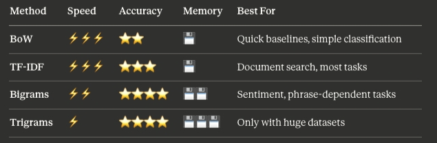
Quick Comparison Table
Decision Guide by Task Type
Task 1: Spam Email Filter
- Recommended: TF-IDF + Logistic Regression
- Why: Clear keyword patterns (“urgent,” “prize,” “click here”)
- Alternative: BoW if speed is absolutely critical
- Avoid: Trigrams (overkill, too sparse)
Task 2: Product Review Sentiment
- Recommended: TF-IDF with bigrams
- Why: Captures negation (“not good”) and intensifiers (“very bad”)
- Alternative: Just TF-IDF if the dataset is small
- Avoid: BoW (will miss negations)
Task: Document Search/Similarity
- Recommended: TF-IDF
- Why: Designed exactly for this — ranks by term importance
- Alternative: None — TF-IDF is the standard
- Avoid: BoW (all words weighted equally)
Task: Topic Classification
- Recommended: TF-IDF
- Why: Different topics have different vocabularies
- Alternative: BoW if topics are very distinct
- Avoid: N-grams (adds complexity without much gain)
Task: Short Text (tweets, chat)
- Recommended: BoW or TF-IDF with careful preprocessing
- Why: Not enough text for reliable TF-IDF statistics
- Alternative: Character n-grams
- Avoid: Word trigrams (way too sparse)
Common Mistakes to Avoid
Mistake 1: Starting with the most complex method
❌ "I'll use trigrams because more context is better"
✅ "I'll start with TF-IDF, measure performance, then add bigrams if needed"
Mistake 2: Not considering production constraints
❌ "This works great on my laptop (takes 10 seconds per prediction)"
✅ "Can this handle 1000 requests/second in production?"
Mistake 3: Ignoring interpretability
❌ "Trigrams give 2% better accuracy, let's use them"
✅ "Can I explain to my manager why this classified a customer email wrong?"
Quick Checklist: Have You Chosen Right?
Before implementing, ask:
✅ Did I try TF-IDF first as a baseline?
✅ Is my method appropriate for my data size?
✅ Can I explain why this method fits my task?
✅ Have I considered production constraints (speed, memory)?
✅ Am I adding complexity only when simpler methods failed?
✅ Can I debug and explain the results to stakeholders?
5. Final Thoughts
When I started learning NLP, I thought I needed to jump straight to neural embeddings or BERT to build anything useful. I was completely wrong.
Frequency-based methods (BoW, TF-IDF, N-grams) are surprisingly powerful. They solve real problems, run fast, and just work.
What I’ve Learned
- TF-IDF beats more complex methods when the vocabulary is distinctive
- Always get a TF-IDF baseline first
- Only move to complex methods if accuracy isn’t acceptable
- Measure everything — don’t assume complexity helps
- Speed, memory, and interpretability matter as much as accuracy
- 90% accuracy with 10ms latency often beats 95% with 1s latency
- Being able to explain decisions has real business value
What’s Next
We’ve covered the foundation — frequency-based embeddings.
In Part 2, we’ll explore neural embeddings (Word2Vec, GloVe, FastText)
6. Resources & Further Learning
- CountVectorizer (Bag-of-Words) : https://scikit-learn.org/stable/modules/generated/sklearn.feature_extraction.text.CountVectorizer.html
Kaggle Notebook: https://www.kaggle.com/code/anucool007/multi-class-text-classification-bag-of-words - TfidfVectorizer (TF-IDF) : https://scikit-learn.org/stable/modules/generated/sklearn.feature_extraction.text.TfidfVectorizer.html
Kaggle Notebook: https://www.kaggle.com/code/viroviro/sentiment-analysis-tf-idf-logistic-regression#Vectorization - Complete Text Feature Extraction Guide : https://scikit-learn.org/stable/modules/feature_extraction.html#text-feature-extraction
Kaggle Notebook: https://www.kaggle.com/code/thecobbler/n-grams-and-bi-grams
#NLP #WordEmbeddings #MachineLearning #AI #TFIDF #BagOfWords #DataScience #Python #TextMining
Word Embeddings in NLP: From Bag-of-Words to Transformers (Part 1) was originally published in Towards AI on Medium, where people are continuing the conversation by highlighting and responding to this story.