
What Actually Breaks ML Models in Production: A Fintech Case Study
Subtitle: Real production incidents from fintech classification models — and the engineering fixes that actually worked
Introduction: The Silent Failures Nobody Talks About
Your model just went live. Training metrics looked great — 0.92 AUC, precision and recall perfectly balanced. The deployment pipeline ran without a single error.
Two weeks later, your product manager sends a Slack message: “Why are we rejecting 40% more applications than last month?”
You check the monitoring dashboard. Everything shows green. The model is running. Predictions are being generated. No exceptions logged.
This is what most ML production failures actually look like.
They don’t crash. They don’t throw errors. They just quietly start making worse decisions, and by the time anyone notices, thousands of predictions have already gone wrong.
After working on multiple fintech classification models — credit risk, fraud detection, loan approvals — I’ve seen the same patterns repeat. This article documents the actual production incidents we encountered, why they were invisible to traditional monitoring, and what engineering practices actually prevented them from happening again.
These aren’t theoretical failure modes from research papers. These are real problems that cost real money and damaged real user experiences.
Failure #1: Training–Serving Skew (When Your Model Lives in Two Different Worlds)
The Incident
A credit risk model started assigning unexpectedly high risk scores to new users. Approval rates dropped by 15% over three weeks. The strange part? Our offline evaluation metrics hadn’t changed at all.
The model wasn’t broken. The features were.
What Was Really Happening
During training, we computed features using complete historical datasets. In production, we computed them using whatever data was actually available at decision time.
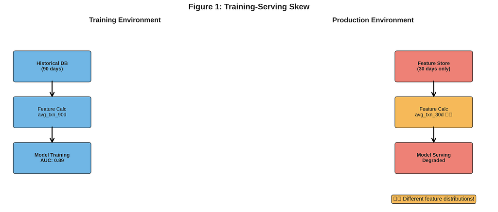
Consider a feature like “average transaction amount over the past 90 days”:
Training environment:
- Full transaction history available
- Feature computed from complete 90-day windows
- Missing data filled using forward-fill or interpolation
Production environment:
- Real-time feature store with 30-day retention
- New users had only 5–10 days of history
- No imputation logic at inference time
The feature had the same name in both environments. It absolutely did not have the same distribution.
The Architecture Problem
┌─────────────────────────────────────────────────────────────┐
│                     TRAINING PIPELINE                        │
│                                                              │
│  Historical DB → Feature Engineering → Model Training       │
│  (complete data)   (90-day windows)     (learns patterns)   │
└─────────────────────────────────────────────────────────────┘
┌─────────────────────────────────────────────────────────────┐
│                   PRODUCTION PIPELINE                        │
│                                                              │
│  Feature Store → Feature Retrieval → Model Inference        │
│  (30-day cache)  (partial windows)   (expects 90d data)     │
└─────────────────────────────────────────────────────────────┘
The model was trained on one distribution and served predictions on a completely different one.
Why Traditional Monitoring Missed It
Our monitoring tracked:
- API latency ✓
- Error rates ✓
- Prediction volume ✓
- Model version ✓
What it didn’t track:
- Feature distribution shifts
- Input data availability
- Computation path differences
The model was technically “working” — it just wasn’t working correctly.
The Code That Caused It
Offline training code:
# Training feature computation
def compute_features_offline(user_transactions_df):
    """
    Uses full historical data from data warehouse
    """
    features = user_transactions_df.groupby('user_id').agg({
        'amount': ['mean', 'std', 'min', 'max'],
        'transaction_date': 'count'
    }).reset_index()

    # Compute rolling statistics with full lookback
    features['avg_amount_90d'] = (
        user_transactions_df
        .sort_values('transaction_date')
        .groupby('user_id')['amount']
        .rolling(window=90, min_periods=1)
        .mean()
        .reset_index(level=0, drop=True)
    )

    return features
Online inference code:
# Production feature computation
def compute_features_online(user_id, feature_store):
    """
    Uses real-time feature store with limited retention
    """
    # Feature store only retains 30 days
    recent_txns = feature_store.get_transactions(
        user_id=user_id,
        days_back=30  # ← This is the problem
    )

    if len(recent_txns) == 0:
        return default_features()

    features = {
        'avg_amount_90d': recent_txns['amount'].mean(),  # Wrong!
        'txn_count': len(recent_txns),
        # ... other features
    }

    return features
Notice the disconnect? The training code expected 90 days. The production code could only provide 30.
What Actually Fixed It
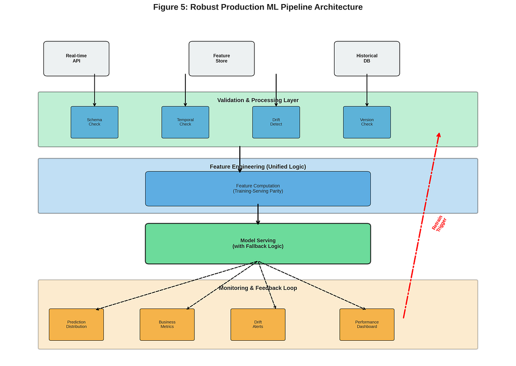
1. Unified Feature Computation
We created a single source of truth for feature definitions:
# Shared feature library
class TransactionFeatures:
    """
    Single feature definition used in both training and serving
    """
    LOOKBACK_WINDOW = 30  # Explicitly defined

    @staticmethod
    def compute_avg_amount(transactions_df):
        """
        Same logic runs in training and production
        """
        if len(transactions_df) == 0:
            return 0.0

        # Filter to exact window used in production
        cutoff_date = datetime.now() - timedelta(days=LOOKBACK_WINDOW)
        recent = transactions_df[
            transactions_df['transaction_date'] >= cutoff_date
        ]

        return recent['amount'].mean() if len(recent) > 0 else 0.0
2. Feature Availability Documentation
We documented what data was actually available at inference time:
FEATURE_DEFINITIONS = {
    'avg_amount_30d': {
        'description': 'Average transaction amount',
        'lookback_days': 30,
        'availability': 'real-time',
        'min_data_points': 3,
        'fallback_value': 0.0
    }
}
3. Training-Serving Consistency Tests
We added automated tests that compared feature distributions:
def test_feature_consistency():
    """
    Verify training and serving features match
    """
    # Generate features using training pipeline
    training_features = compute_features_offline(sample_users)

    # Generate same features using production pipeline
    serving_features = [
        compute_features_online(user_id, feature_store)
        for user_id in sample_users
    ]

    # Compare distributions
    for feature_name in FEATURE_DEFINITIONS.keys():
        train_dist = training_features[feature_name]
        serve_dist = [f[feature_name] for f in serving_features]

        # Statistical comparison
        ks_stat, p_value = ks_2samp(train_dist, serve_dist)

        assert p_value > 0.05, (
            f"Feature {feature_name} distributions differ: "
            f"KS statistic = {ks_stat}, p-value = {p_value}"
        )
4. Feature Removal Over Feature Engineering
In several cases, we simply removed problematic features:
- Features requiring data unavailable at inference time → Removed
- Features with inconsistent computation paths → Removed
- Features that couldn’t be reliably replicated → Removed
Counterintuitively, removing features improved production stability more than trying to “fix” them with complex imputation strategies.
The Real Lesson
Training-serving skew isn’t a model problem. It’s an engineering problem.
The model trained correctly. The deployment succeeded. The infrastructure worked. But the data pipeline assumptions were fundamentally incompatible between environments.
The fix wasn’t better models. It was better data engineering.
Failure #2: Data Drift That Monitoring Couldn’t See
The Incident
A fraud detection model started flagging legitimate transactions as suspicious. False positive rate jumped from 3% to 12% over six weeks. Customer complaints increased proportionally.
Our drift detection showed… nothing unusual.
What Changed
The model’s input distribution hadn’t drifted. The world had drifted.
A major payment processor changed their transaction metadata format. What was previously a categorical field with 50 distinct values suddenly had 200+ values. Our model had never seen most of them during training.
The Architecture Gap
┌──────────────────────────────────────────────────────────┐
│                  TRAINING DATA (2022-2023)                │
│                                                           │
│  Transaction Category: ['retail', 'food', 'gas', ...]   │
│  Total unique values: 50                                 │
│  Coverage: 99.8% of transactions                         │
└──────────────────────────────────────────────────────────┘
┌──────────────────────────────────────────────────────────┐
│              PRODUCTION DATA (March 2024)                 │
│                                                           │
│  Transaction Category: ['retail', 'food', 'gas', ...]   │
│  + 150 NEW values from payment processor update          │
│  Coverage: 60% of transactions match training            │
└──────────────────────────────────────────────────────────┘

Why Standard Drift Detection Failed
Our drift monitoring compared statistical distributions:
# Standard drift detection
def detect_drift(reference_data, production_data, feature_name):
    """
    Compares distributions using KL divergence
    """
    ref_dist = reference_data[feature_name].value_counts(normalize=True)
    prod_dist = production_data[feature_name].value_counts(normalize=True)

    kl_div = entropy(ref_dist, prod_dist)

    return kl_div > DRIFT_THRESHOLD
The problem? For categorical features with many new values, KL divergence doesn’t capture the semantic shift effectively. The distribution might look similar statistically while being completely different semantically.
What Actually Fixed It
1. Vocabulary Monitoring
Track which values the model has actually seen:
class VocabularyMonitor:
    def __init__(self, training_vocab):
        self.known_values = set(training_vocab)

    def check_production_value(self, value):
        """
        Flag unknown categorical values
        """
        if value not in self.known_values:
            logging.warning(
                f"Unknown categorical value encountered: {value}"
            )
            return False
        return True

    def get_coverage(self, production_data):
        """
        Calculate percentage of known values
        """
        total = len(production_data)
        known = sum(
            val in self.known_values
            for val in production_data
        )
        return known / total
2. Semantic Drift Detection
Instead of just comparing distributions, we monitored coverage:
def monitor_categorical_coverage(feature_name, production_batch):
    """
    Track how many production values were seen during training
    """
    training_values = get_training_vocabulary(feature_name)

    production_values = set(production_batch[feature_name].unique())

    coverage = len(
        production_values & training_values
    ) / len(production_values)

    if coverage < 0.8:  # Alert threshold
        alert(
            f"Only {coverage*100:.1f}% of production "
            f"values were seen during training"
        )
3. Graceful Unknown Handling
Default handling for unseen categorical values:
def encode_categorical_safe(value, known_encodings):
    """
    Handle unknown categorical values gracefully
    """
    if value in known_encodings:
        return known_encodings[value]
    else:
        # Map to 'unknown' category instead of crashing
        return known_encodings.get('__UNKNOWN__', 0)
The Real Lesson
Drift detection isn’t just about distribution statistics. It’s about tracking what your model has actually learned.
For categorical features, monitoring vocabulary coverage matters more than monitoring statistical moments.
Failure #3: Label Leakage Discovered After Deployment
The Incident
A loan default prediction model achieved 0.96 AUC during training. After deployment, it was essentially useless — barely better than random guessing.
We had label leakage. And it only became obvious in production.
What Leaked
One of our features was “days since last payment.” During training, we computed this using the full transaction history — including transactions that occurred after the loan default.
In production, we could only compute it using data available before the prediction.
The Subtle Bug
Training code:
# This runs on historical data
def compute_days_since_last_payment(user_id, reference_date):
    """
    Computes using ALL historical data
    """
    all_payments = get_all_payments(user_id)  # Includes future!

    payments_before_ref = all_payments[
        all_payments['date'] <= reference_date
    ]

    if len(payments_before_ref) == 0:
        return 999  # Large default value

    last_payment = payments_before_ref['date'].max()

    return (reference_date - last_payment).days
The problem isn’t obvious until you realize get_all_payments() returned the complete payment history, including payments made after the default date.

What should have been:
def compute_days_since_last_payment(user_id, reference_date):
    """
    Computes using only data available at reference_date
    """
    # Only get payments BEFORE the reference date
    payments = get_payments_before_date(user_id, reference_date)

    if len(payments) == 0:
        return 999

    last_payment = payments['date'].max()

    return (reference_date - last_payment).days
Why This Went Undetected
Cross-validation looked perfect because the leakage was consistent across train/validation splits. The model learned a pattern that was only valid when future data was available.
What Actually Fixed It
1. Point-in-Time Feature Engineering
We enforced strict temporal boundaries:
class PointInTimeFeatureStore:
    """
    Ensures features only use data available at decision time
    """
    def get_features(self, user_id, as_of_date):
        """
        as_of_date: The decision timestamp
        """
        # Hard constraint: no data after as_of_date
        historical_data = self.db.query(
            f"""
            SELECT * FROM transactions
            WHERE user_id = {user_id}
            AND transaction_date < '{as_of_date}'
            """
        )

        return self.compute_features(historical_data)
2. Production-First Feature Development
We reversed the development process:
- First: Write the production feature computation code
- Second: Replay it on historical data for training
- Third: Validate that both paths produce identical results
# Define production logic first
def production_feature_logic(data_before_decision):
    return {
        'days_since_last_payment': compute_payment_recency(data_before_decision),
        'total_transactions': len(data_before_decision),
        # ... other features
    }
# Use the same logic for training
def create_training_dataset(historical_users, decision_dates):
    """
    Replay production logic on historical data
    """
    features = []

    for user_id, decision_date in zip(historical_users, decision_dates):
        # Get data exactly as production would see it
        data_available = get_data_before_date(user_id, decision_date)

        # Use the exact same feature computation
        user_features = production_feature_logic(data_available)

        features.append(user_features)

    return pd.DataFrame(features)
The Real Lesson
Label leakage isn’t just a data science problem. It’s a time-travel problem.
If your training features use any information that wouldn’t be available at prediction time, your model is learning to predict the past, not the future.
What Actually Prevents These Failures: The Engineering Practices That Worked
After fixing these incidents multiple times, a clear pattern emerged. The solutions weren’t about better algorithms or more sophisticated monitoring. They were about engineering discipline.
Practice 1: Feature Contracts
Treat features like API contracts:
# feature_definitions.yaml
features:
  avg_transaction_amount_30d:
    description: "Average transaction amount over last 30 days"
    data_source: "transactions table"
    lookback_window: 30
    minimum_data_points: 3
    fallback_value: 0.0
    computation:
      training: "features.offline.compute_avg_amount()"
      serving: "features.online.compute_avg_amount()"
    validation:
      - name: "distribution_match"
        threshold: 0.05
      - name: "null_rate"
        threshold: 0.01
Practice 2: Unified Feature Repositories
One codebase for both training and serving:
feature_repo/
├── __init__.py
├── base.py          # Abstract feature interface
├── transaction.py   # Transaction features
├── user.py          # User features
└── tests/
    ├── test_consistency.py
    └── test_distributions.py

Practice 3: Production-First Development
Step 1: Design feature for production constraints
        ↓
Step 2: Implement production feature computation
        ↓
Step 3: Replay production logic on historical data
        ↓
Step 4: Train model using replayed features
        ↓
Step 5: Validate training/serving consistency
Practice 4: Continuous Validation
# Runs every hour in production
def validate_production_features():
    """
    Automated checks for training-serving consistency
    """
    # Sample recent production requests
    prod_samples = sample_recent_predictions(n=1000)

    # Recompute using training logic
    training_features = compute_offline_features(prod_samples)

    # Compare
    for feature in FEATURE_LIST:
        prod_values = prod_samples[feature]
        train_values = training_features[feature]

        # Statistical comparison
        assert_distributions_match(prod_values, train_values)

        # Null rate comparison
        assert_null_rates_match(prod_values, train_values)
Conclusion: Production ML Is an Engineering Problem
The biggest lesson from these failures is simple: most ML production issues aren’t ML issues.
They’re engineering issues that happen to involve ML models:
- Training-serving skew is a data pipeline problem
- Data drift is a monitoring problem
- Label leakage is a temporal consistency problem
The models themselves were fine. The math was correct. The algorithms worked. What failed was the infrastructure around them.
If you’re building production ML systems, invest more time in:
- Feature engineering discipline
- Training-serving consistency
- Temporal correctness
- Automated validation
And less time in:
- Chasing marginal accuracy improvements
- Complex model architectures
- Hyperparameter tuning
The model that deploys reliably is better than the model that performs slightly better in offline evaluation.
References and Further Reading
- Sculley et al. (2015) — “Hidden Technical Debt in Machine Learning Systems”
- Google’s “Rules of Machine Learning” — #5: Test the infrastructure independently from the model
- Feast Feature Store Documentation — Consistency Guarantees
Thanks for reading! If you’ve encountered similar production failures or have questions about these fixes, I’d love to hear from you in the comments.
What Actually Breaks ML Models in Production: A Fintech Case Study was originally published in Towards AI on Medium, where people are continuing the conversation by highlighting and responding to this story.