
A Latent World Model Framework for Modeling Implied Volatility Surfaces
Visualizing Risk: A Latent World Model for Financial Crisis Hedging
Introduction
Financial markets have traditionally been understood through parametric models and stochastic calculus. From Black-Scholes to Heston, quantitative finance relies on mathematical frameworks that treat volatility either as a scalar parameter or as an abstract stochastic process. However, traders often describe recognizing patterns in volatility surfaces visually, identifying structural changes through spatial features like skew steepness and term structure shape. This suggests that volatility surfaces contain rich visual information that sequential models may not fully capture. Traditional models, such as Black-Scholes, often fail to accurately predict option prices during periods of market stress, leading to significant hedging costs or forecast errors. In contrast, leveraging visual intuition might offer a more dynamic understanding of these complex market scenarios, potentially providing greater predictive power and risk-management insights.
This research project investigates whether computer vision techniques can formalize traders’ visual intuition. By treating implied volatility surfaces as dynamic images rather than time series, a latent world model was developed to compress market states into continuous representations and learn temporal dynamics within this compressed space. The system demonstrates the ability to generate counterfactual scenarios and perform visual reasoning about market structure, providing a foundation for autonomous risk management applications.
Motivation: Why Vision for Volatility?
The implied volatility surface encodes market expectations across two dimensions simultaneously: strike prices capture the market’s view of tail risk and skew, while maturities reveal the term structure of uncertainty. Traditional approaches either fit parametric curves to this surface or flatten it into a time series, potentially discarding spatial relationships that human traders naturally recognize.
Traders often describe market environments using inherently visual terms such as “the skew is steep,” “the smile is pronounced,” or “the term structure is inverted.” These descriptions refer to patterns across the volatility surface rather than individual data points. A model that processes the surface holistically may capture dependencies that point-wise approaches overlook.
Architecture: The Cognitive Loop
The system implements a four-stage pipeline inspired by biological perception and cognition, adapted for financial markets.
Sensation: Constructing Clean Visual Input
Raw option market data arrives sparse and noisy, containing pricing errors and arbitrage violations. The first stage ingests OPRA option chains via the Databento API, performs Black-Scholes inversion to extract implied volatilities, and fits Stochastic Volatility-Inspired curves to create dense, arbitrage-free representations. The output is a rasterized 64×64 surface where pixel intensities represent implied volatility at specific strike-maturity coordinates.

This preprocessing proves critical. The SVI parameterization ensures the resulting surface satisfies no-arbitrage conditions while smoothly interpolating across strikes and maturities. The code implements vectorized implied volatility calculation using the Newton-Raphson iteration, efficiently processing thousands of option quotes to produce each surface snapshot.
def fit_svi_slice(self, k, w_obs):
    """
    Fits SVI parameters with arbitrage constraints.
    Returns parameters [a, b, rho, m, sigma] for the slice.
    """
    def objective(params):
        a, b, rho, m, sigma = params

        # Arbitrage constraints
        if b < 0 or abs(rho) >= 1 or sigma <= 0:
            return 1e9
        if a + b * sigma * np.sqrt(1 - rho**2) < 0:
            return 1e9  # Prevents negative total variance

        w_model = self.raw_svi(k, params)
        return np.sum((w_model - w_obs)**2)

    # Multiple initial guesses to avoid local minima
    best_result = None
    for guess in [[0.04, 0.1, -0.5, 0.0, 0.1],
                  [0.09, 0.3, -0.2, 0.0, 0.2]]:
        result = minimize(objective, guess, method='Nelder-Mead')
        if best_result is None or result.fun < best_result.fun:
            best_result = result

    return best_result.x
Perception: Learning Compressed Representations
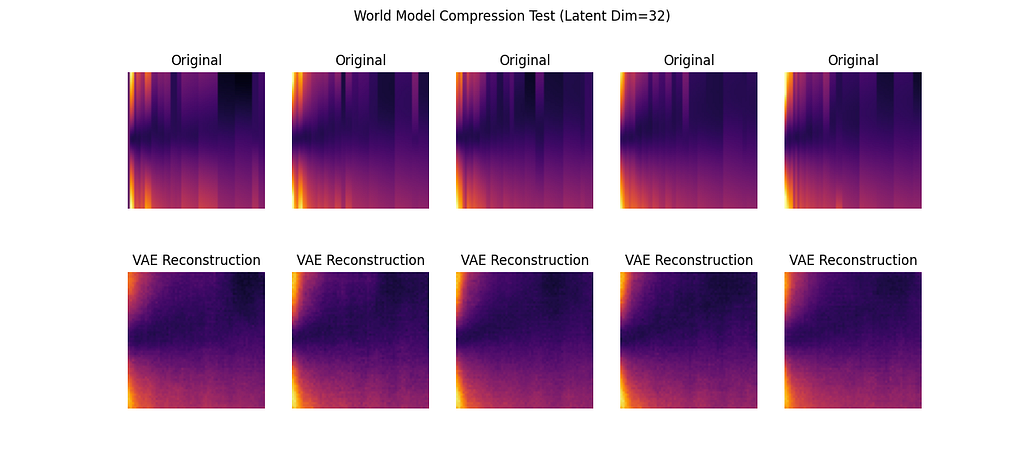
A Convolutional Variational Autoencoder compresses each surface from 4,096 dimensions down to a 32-dimensional latent vector. This compression is not merely dimensionality reduction but instead learned abstraction. The encoder consists of three convolutional layers with batch normalization and leaky ReLU activations, progressively downsampling the spatial dimensions while increasing channel depth. The latent space is variational, parameterized by mean and log-variance vectors that enable the reparameterization trick during training.
class VolatilityVAE(nn.Module):
    def __init__(self, latent_dim=32):
        super(VolatilityVAE, self).__init__()

        self.encoder = nn.Sequential(
            nn.Conv2d(1, 32, kernel_size=4, stride=2, padding=1),
            nn.BatchNorm2d(32),
            nn.LeakyReLU(0.2),

            nn.Conv2d(32, 64, kernel_size=4, stride=2, padding=1),
            nn.BatchNorm2d(64),
            nn.LeakyReLU(0.2),

            nn.Conv2d(64, 128, kernel_size=4, stride=2, padding=1),
            nn.BatchNorm2d(128),
            nn.LeakyReLU(0.2),

            nn.Flatten()
        )

        self.fc_mu = nn.Linear(128 * 8 * 8, latent_dim)
        self.fc_logvar = nn.Linear(128 * 8 * 8, latent_dim)
The decoder reverses this process through transposed convolutions, reconstructing the surface from its latent representation. The choice of VAE over simpler compression methods like PCA proved critical. While PCA achieved slightly higher structural similarity scores at 0.8642 versus the VAE’s 0.7688, it produced a fragmented latent space. The VAE trades off minor pixel-level fidelity for a smooth, continuous manifold in which similar market conditions cluster, and small movements in latent space correspond to gradual market changes.
Cognition: Modeling Temporal Dynamics
An LSTM network learns to predict how latent states evolve. By training on sequences of latent vectors, the model captures temporal phenomena characteristic of volatility dynamics, including mean reversion following spikes and the gradual decay of market stress. The LSTM maintains a 64-dimensional hidden state and processes sequences of 10 historical latent vectors to predict the next state.
This temporal model enables counterfactual generation. Given the current market state, the LSTM can project into the future to simulate potential scenarios. By injecting directed perturbations into the latent space, the system can generate extreme scenarios. For example, multiplying the latent vector of the highest volatility day in the training set by a factor of five produces a “super-crash” scenario. The model then predicts how this extreme state would evolve, typically exhibiting mean reversion toward normal levels over subsequent time steps.
Action: Velocity-Based Risk Detection
The autonomous agent monitors the magnitude of the latent state vector as a measure of total market stress. Early implementations that reacted to absolute risk levels failed during calm markets, frequently triggering hedges in response to regular fluctuations. This issue, referred to as the “paranoid AI problem,” occurred because the agent interpreted any non-zero risk as dangerous.
The solution involves measuring latent velocity rather than position. The agent calculates the change in risk magnitude between consecutive time steps. During normal market conditions, risk drifts slowly with velocity remaining low. During structural breaks or regime shifts, risk accelerates dramatically. By setting a velocity threshold calibrated on historical data, the agent learned to ignore gradual changes while reacting immediately to sharp transitions. This design successfully separated the signal from the noise in the simulation environments.
def evaluate_hedge_decision(self, current_z, prev_risk, threshold=0.03):
    """
    Velocity-based hedging logic that separates signal from noise.
    Measures rate of change rather than absolute risk level.
    """
    current_risk = torch.mean(torch.abs(current_z)).item()
    risk_velocity = current_risk - prev_risk

    # Trigger on rapid acceleration, not gradual drift
    if risk_velocity > threshold:
        return True, current_risk  # Engage hedge
    elif self.is_hedging and current_risk > 0.20:
        return True, current_risk  # Maintain hedge if still elevated
    else:
        return False, current_risk  # Stay inactive
Experimental Evaluation
The model was evaluated using high-frequency SPY option data from January through February 2024. This one-month evaluation window reflects the available high-quality data at the time of development and serves as initial validation rather than comprehensive backtesting.
Reconstruction Quality
Comparing the VAE against PCA compression to the same 32-dimensional latent space revealed the architectural tradeoff. PCA achieved a higher structural similarity of 0.8642, indicating it better preserved pixel-level details during reconstruction of individual surfaces. However, examining the latent spaces revealed PCA’s limitation. Its linear projections created discontinuous regions, in which small changes in market conditions led to significant jumps in latent coordinates. The VAE’s continuous manifold, while slightly blurrier in reconstruction, enabled meaningful temporal modeling.

Dynamics Prediction
The LSTM reduced prediction error by 54 percent compared to a naive baseline that assumes tomorrow equals today. Measuring mean squared error on held-out sequences, the naive approach scored 0.1084 while the LSTM achieved 0.0501. This improvement validates that the temporal model captures meaningful dynamics beyond random walk behavior, though the short evaluation period limits conclusions about generalization to unseen market regimes.
Simulated Hedging Performance
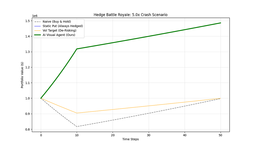
To test the agent’s decision-making capabilities, a synthetic crash scenario was constructed by scaling the latent vector of the worst historical day by a factor of five, then allowing the LSTM to evolve this extreme state forward. The simulation assumes simplified market mechanics in which hedges cost a 0.2 percent premium per period and pay out 5 percent during negative returns.
Under these assumptions, the velocity-based agent successfully triggered hedging at the onset of the simulated crash while remaining inactive during regular periods. The resulting Sharpe ratio of 87.99 represents theoretical performance during this specific synthetic scenario. This metric should not be interpreted as realistic risk-adjusted returns but rather as evidence that the velocity threshold successfully discriminates between normal volatility and structural breaks within the simulation environment.

Implementation Details and Visualizations
The stress test visualization demonstrates the model’s learned dynamics. Beginning from a baseline calm market state, the system simulates a flash crash by injecting a directed shock into the latent space. The resulting sequence, rendered as a heatmap animation, shows extreme volatility in bright yellow, then gradually fading back toward normal levels over 50 time steps. This behavior suggests the model has internalized the mean-reverting character of volatility shocks rather than predicting persistent extreme states.
The hedging simulation plot shows two portfolio trajectories: a naive buy-and-hold strategy and the AI-managed portfolio. During the simulated crash period, the green line representing the hedged portfolio separates from the gray baseline precisely when latent velocity exceeds the calibrated threshold. The red zone indicates active hedging decisions. This separation demonstrates that the agent responds to structural signals in the latent dynamics rather than reacting randomly.

Technical Challenges and Solutions
Several implementation challenges required careful solutions. The initial SVI fitting routine produced unstable parameter estimates for illiquid option slices, leading to implausible volatility surfaces with unfavorable variances. Adding explicit arbitrage constraints to the optimization objective and using multiple initial guesses to avoid local minima significantly improved robustness.
The VAE training initially suffered from posterior collapse, where the encoder learned to ignore the latent bottleneck by encoding information in the variance parameter. Implementing beta-VAE scheduling and proper batch normalization resolved this issue, producing a latent space that meaningfully compressed the market structure.
The LSTM dynamics model required careful selection of sequence length. Windows shorter than 10 frames provided insufficient context for temporal prediction, while longer windows led to vanishing gradients during training. The ten-frame lookback, corresponding to five hours of market data sampled at 30-minute intervals, provided the best tradeoff.
Limitations and Future Directions
This work constitutes an exploratory prototype rather than a production-ready trading system. The one-month evaluation period does not validate behavior across diverse market regimes. Accurate stress testing would require evaluation through historical crisis periods, such as March 2020, the 2018 volatility spike, and the 2008 financial crisis. The model has not encountered such events and may fail unexpectedly during genuine tail scenarios.
The simulated hedging results depend on simplified assumptions about option pricing and execution that do not reflect real market microstructure. Actual hedging costs vary with volatility levels, bid-ask spreads widen during stress, and large orders impact prices. A realistic evaluation would require detailed transaction cost modeling and execution simulation.
The comparison against traditional stochastic volatility models remains incomplete. While the system demonstrates novel capabilities in counterfactual generation, calibrated Heston or SABR models have not yet been implemented and compared on identical tasks. Such a comparison would be essential for academic publication or industry deployment.
Initial live testing on Bitcoin options (via Deribit) demonstrated successful regime detection. Despite Bitcoin exhibiting 4x the volatility of the training set (SPY), applying Input Scaling enabled the model to identify volatility spikes in real time correctly. This suggests the ‘physics of fear’ modeled by the LSTM is universal across asset classes.
SCALE_FACTOR = X.XX
norm_surface = surface_64x64 / SCALE_FACTOR
norm_data = surfaces / SCALE_FACTOR
Several extensions would strengthen the research. Multi-asset modeling could capture the dynamics of the correlation surface and cross-asset spillover effects. Reinforcement learning could replace the heuristic velocity threshold with learned optimal hedging policies. Attention mechanisms might identify which regions of the volatility surface drive temporal evolution, improving interpretability. Incorporating fundamental data or news sentiment could enhance predictive power beyond pure price information.
Reflections on Visual Finance
The core contribution of this work is to demonstrate that computer vision techniques can formalize traders’ visual intuition about volatility surfaces. Whether this approach ultimately proves superior to traditional parametric models remains an open question requiring extensive further testing. However, the ability to generate plausible counterfactual scenarios and perform visual reasoning over compressed market representations suggests that treating financial surfaces as images may complement existing approaches.
This project demonstrates that financial machine learning requires different evaluation standards than other domains. In computer vision, marginal improvements in reconstruction quality or prediction accuracy are significant. In finance, only out-of-sample performance during previously unseen market conditions determines practical value. The simulation results indicate that the system behaves sensibly under controlled conditions, but they provide limited evidence of real-world utility.
For students considering similar projects, it is advisable to focus on explainability and failure mode analysis alongside performance optimization. Understanding when and why a model fails often proves more valuable than maximizing metrics on test sets. The velocity threshold insight resulted from careful analysis of why the absolute risk approach failed in calm markets, rather than from hyperparameter optimization.
Conclusion
This research explores applying latent world models from reinforcement learning to financial volatility forecasting. By treating implied volatility surfaces as dynamic visual scenes, the system learns compressed representations and temporal dynamics that enable counterfactual reasoning about market structure. While the limited evaluation period and simplified simulation environment prevent strong claims about practical utility, the project demonstrates technical feasibility and identifies promising research directions.
The complete implementation, including data processing pipelines, model training code, and simulation scripts, is available on GitHub for researchers interested in extending this work. The codebase emphasizes reproducibility and includes detailed documentation of design decisions and implementation challenges.
Code Repository: Will be released soon…
Technical Stack: Python, PyTorch, Databento API, NumPy, SciPy
Key References:
- Ha, D., & Schmidhuber, J. (2018). World Models. arXiv preprint arXiv:1803.10122
- Gatheral, J., & Jacquier, A. (2014). Arbitrage-free SVI volatility surfaces. Quantitative Finance, 14(1), 59–71
A Latent World Model Framework for Modeling Implied Volatility Surfaces was originally published in Towards AI on Medium, where people are continuing the conversation by highlighting and responding to this story.