Beyond Gradient Descent: A Practical Guide to SGD, Momentum, RMSProp, and Adam (with Worked…

Beyond Gradient Descent: A Practical Guide to SGD, Momentum, RMSProp, and Adam (with Worked Examples)

When we train machine learning models, we rarely use “vanilla” gradient descent. In practice, we almost always reach for improved variants that converge faster, behave better with noisy gradients, and handle tricky loss landscapes more reliably. Modern training commonly relies on stochastic gradient descent (mini-batch SGD), plus optimizers like Momentum, RMSProp, and Adam.

1) The baseline: Gradient Descent vs. Stochastic (Mini-batch) Gradient Descent

1.1 What vanilla gradient descent does

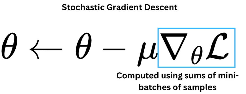
Suppose we want to minimize a loss function L(θ) with parameters θ. Vanilla gradient descent updates parameters using the full dataset:

θ←θ−μ∇θ​L(θ)

• μ is the learning rate
• ∇θ​L is the gradient of the loss w.r.t parameters

Issue: computing gradients over the entire dataset each step can be slow.

1.2 Mini-batch SGD: the practical workhorse

Instead of using all samples, mini-batch SGD estimates the gradient using a small batch (e.g., 32/64/128). This gives faster iterations and often helps the optimizer explore the loss surface better. SGD (in practice, mini-batch SGD) improves convergence by computing loss/gradients on mini-batches.

2) A tiny dataset we’ll use for all worked examples

We’ll use a simple linear regression with one feature:

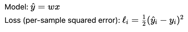
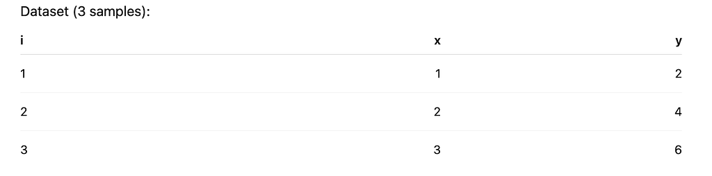
This dataset is perfectly linear: the best w is 2.

Gradient for one sample:

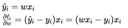
We’ll start at w_0 = 0 and use learning rate μ=0.1.

3) Mini-batch SGD in action (with numbers)

Let’s pick a mini-batch of two samples: (x,y)=(1,2),(2,4)

At w_0 = 0:

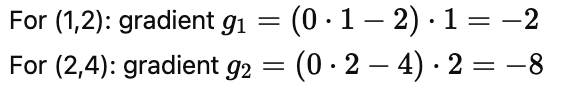
Mini-batch mean gradient:

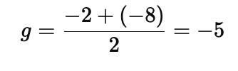
Update:

Interpretation: the negative gradient pushes w upward toward 2.

What can go wrong with plain SGD?

• Gradients vary from batch to batch → updates can be noisy
• If the loss surface has “ravines” (steep in one direction, shallow in another), SGD can zig-zag and slow down

That’s why we introduce Momentum.

4) Momentum: “don’t forget where you were going”

The key weakness of standard SGD: each step reacts to the current gradient and ignores previous steps — so it doesn’t “carry” directionality forward. Momentum fixes that by using an exponential average of past gradients.

4.1 Momentum update rules

Common form:

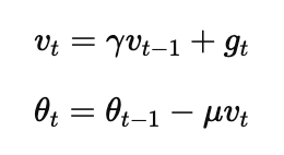
gt is the current mini-batch gradient

γ (often ~0.9) controls how much “memory” we keep

4.2 Worked example (same mini-batch gradient)

Assume:

• μ = 0.1
• γ = 0.9
• Start: w₀ = 0, v₀ = 0
• Batch gradient from earlier: g₁ = −5

Step 1:

• v₁ = 0.9(0) + (−5) = −5
• w₁ = 0 − 0.1(−5) = 0.5

Now imagine the next batch has gradient g₂ = −4 (still pushing upward, consistent direction):

Step 2:

• v₂ = 0.9(−5) + (−4) = −8.5
• w₂ = 0.5 − 0.1(−8.5) = 1.35

Key effect: even though the new gradient is only −4, the velocity accumulates direction, so the step is larger than plain SGD would take.

4.3 When Momentum shines

• Long ravines (common in deep nets): reduces zig-zagging
• Noisy gradients: smooths updates
• Faster convergence when the direction is consistent (exactly as your transcript states)

5) RMSProp: adaptive learning rates to tame exploding/vanishing gradients

RMSProp (Root Mean Square Propagation) adjusts the learning rate per parameter using a moving average of squared gradients. RMSProp’s helps avoiding vanishing/exploding gradients by using an adaptive learning rate.

5.1 RMSProp update rules

Maintain an exponential moving average of squared gradients:

sₜ = βsₜ₋₁ + (1 − β)gₜ²

Then update:

θₜ = θₜ₋₁ − (μ / √(sₜ + ε)) gₜ

• β often ~0.9
• ε is a small number like 10⁻⁸ to avoid divide-by-zero

5.2 What RMSProp is really doing (intuition)

• If recent gradients are large, sₜ becomes large → denominator grows → step size shrinks → prevents runaway updates (exploding behavior).
• If recent gradients are tiny, sₜ stays small → denominator small → step size increases → helps keep learning moving (fights vanishing updates).

5.3 Worked example (one parameter)

Assume:

• μ = 0.1, β = 0.9, ε ≈ 0 (just for easy arithmetic)
• w₀ = 0, s₀ = 0
• First mini-batch gradient g₁ = −5

Compute:

• s₁ = 0.9(0) + 0.1(25) = 2.5
• Effective step multiplier: μ / √s₁ = 0.1 / √2.5 ≈ 0.1 / 1.58 ≈ 0.063

Update:

• w₁ = 0 − (0.063)(−5) ≈ 0.315

Notice: plain SGD jumped to 0.5, but RMSProp damped the step because the gradient magnitude was big.

Now suppose next gradient is smaller: g₂ = −1

• s₂ = 0.9(2.5) + 0.1(1) = 2.35
• step multiplier ≈ 0.1 / √2.35 ≈ 0.065
• update size ≈ 0.065

RMSProp keeps steps stable even as gradients change scale.

6) Adam: Momentum + RMSProp (and bias correction)

Adam is widely used because it blends:

• Momentum-like smoothing via moving average of gradients
• RMSProp-like scaling via moving average of squared gradients

Adam combines momentum and adaptive learning rates.

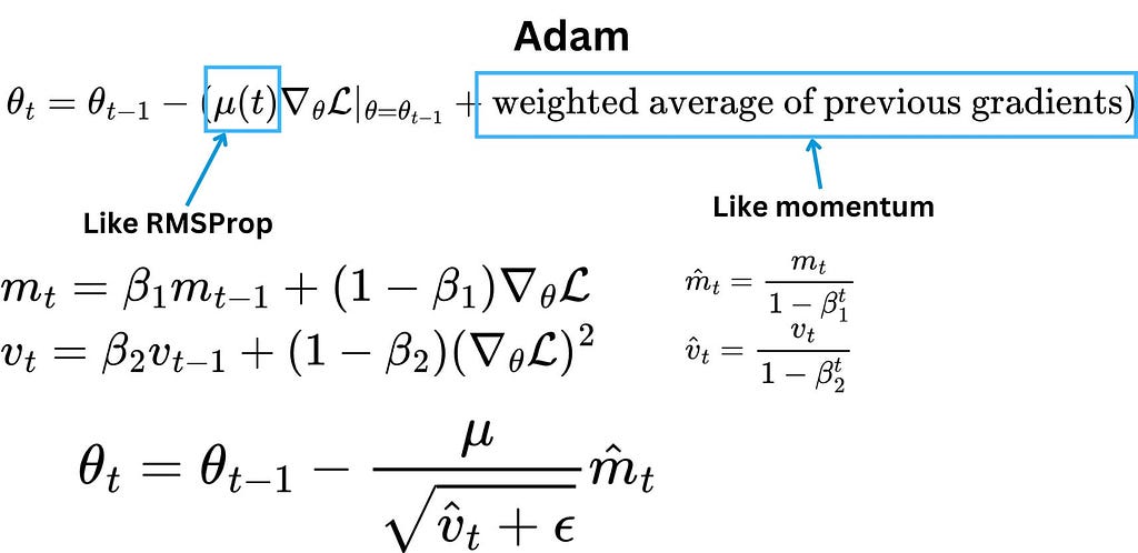
6.1 Adam update rules (standard form)

Adam keeps two moving averages:

First moment (mean of gradients):

mₜ = β₁mₜ₋₁ + (1 − β₁)gₜ

Second moment (mean of squared gradients):

vₜ = β₂vₜ₋₁ + (1 − β₂)gₜ²

Bias correction (important early on):

m̂ₜ = mₜ / (1 − β₁ᵗ), v̂ₜ = vₜ / (1 − β₂ᵗ)

Final update:

θₜ = θₜ₋₁ − (μ / √(v̂ₜ + ε)) m̂ₜ

Typical defaults:

• β₁ = 0.9
• β₂ = 0.999
• ε = 10⁻⁸

6.2 Why bias correction matters (simple intuition)

At t = 1, both m₀ and v₀ start at 0, so the moving averages are biased toward 0 initially. Bias correction removes that “cold start” effect so early updates aren’t artificially small — initial bias toward zero and why correction is crucial early in training.

6.3 Worked example (one step)

Assume:

• μ = 0.1, β₁ = 0.9, β₂ = 0.999
• m₀ = 0, v₀ = 0
• gradient g₁ = −5

Compute moments:

• m₁ = 0.9(0) + 0.1(−5) = −0.5
• v₁ = 0.999(0) + 0.001(25) = 0.025

Bias-correct:

• m̂₁ = −0.5 / (1−0.9¹) = −0.5 / 0.1 = −5
• v̂₁ = 0.025 / (1−0.99⁹¹) = 0.025 / 0.001 = 25

Update:

w₁ = 0 − (0.1 / √25)(−5) = 0 − (0.1 / 5)(−5) = 0.1

What just happened?

• Adam used the gradient direction like momentum (via m̂₁)
• Adam scaled it like RMSProp (via √v̂₁)
• With this setup, the first step is deliberately conservative and scale-normalized

In practice, Adam often feels “easy mode” because it’s less sensitive to gradient scaling across parameters, which is common in deep networks.

7) Choosing between SGD, Momentum, RMSProp, and Adam (practical guidance)

Use mini-batch SGD when:

• You want simplicity and strong baselines
• You’re training convex-ish models or smaller networks
• You plan to tune learning rate schedules carefully

Add Momentum when:

• You see oscillations / zig-zagging
• You want faster convergence along consistent directions
• You’re training CNNs/vision models where SGD+Momentum is still extremely competitive

Use RMSProp when:

• Gradients are noisy or vary wildly in scale
• You need stability against exploding/vanishing update magnitudes
• You’re training RNN-like systems or setups with sparse/noisy gradients (historically common use)

Use Adam when:

• You want strong “out of the box” performance
• You’re working with transformers / large deep nets
• You don’t want to micromanage per-parameter scaling

A very common modern default: Adam (or AdamW) as a starting point, then consider switching to SGD+Momentum for specific tasks where it generalizes better.

8) Minimal “from-scratch” pseudocode (all four)

Here’s a compact view of the mechanics (conceptually; not framework-specific):

# Given gradient g at step t

# SGD:
theta -= lr * g

# Momentum:
v = gamma * v + g
theta -= lr * v

# RMSProp:
s = beta * s + (1 - beta) * (g * g)
theta -= lr * g / (sqrt(s) + eps)

# Adam:
m = beta1 * m + (1 - beta1) * g
v = beta2 * v + (1 - beta2) * (g * g)
m_hat = m / (1 - beta1**t)
v_hat = v / (1 - beta2**t)
theta -= lr * m_hat / (sqrt(v_hat) + eps)

Closing thoughts

All four optimizers are fundamentally answering the same question:

“Given the gradient, how should we step — how far, and in what smoothed/scaled direction — so training is fast and stable?”

• SGD: “step in the gradient direction”
• Momentum: “step in a smoothed, history-aware direction”
• RMSProp: “scale steps to match recent gradient magnitudes”
• Adam: “do both, plus correct early-step bias”

---

Beyond Gradient Descent: A Practical Guide to SGD, Momentum, RMSProp, and Adam (with Worked… was originally published in Towards AI on Medium, where people are continuing the conversation by highlighting and responding to this story.