PCA — Covariance Matrix, Eigen Vector, Eigen value

digitado ⋅ 9 de January de 2026

PCA — Covariance Matrix, Eigen Vector, Eigen value

Why PCA

In machine learning, data is power — but only when we can make sense of it. Most real-world datasets contain many features (also called dimensions or variables). Sometimes, datasets can easily have hundreds or even thousands of features. While abundance might seem advantageous, it presents a significant hurdle for machine learning algorithms.

As the number of features grows, models face several challenges:

Slower Training: More features mean more computations, leading to longer training times.
Difficult Visualization: Humans struggle to visualize data beyond three dimensions, making it hard to grasp underlying patterns.
Pattern Identification Struggles: With too many variables, it becomes harder for algorithms to discern true relationships from noise.

This challenge leads us to a fundamental problem known as the Curse of Dimensionality.

Pattern Identification Struggles: With too many variables, it becomes harder for algorithms to discern true relationships from noise.

This phenomenon is famously known as the Curse of Dimensionality.

Curse of Dimensionality

The Curse of Dimensionality refers to the phenomenon where the difficulty of analyzing data increases as the number of dimensions increases.

As you can see in the picture above, the data becomes more sparse, and the distance between each point increases, as the number of dimensions increases. This makes it harder to find patterns or relationships in the data.

How to Handle Curse of Dimensionality

Some of the ways to handle curse of dimensionality

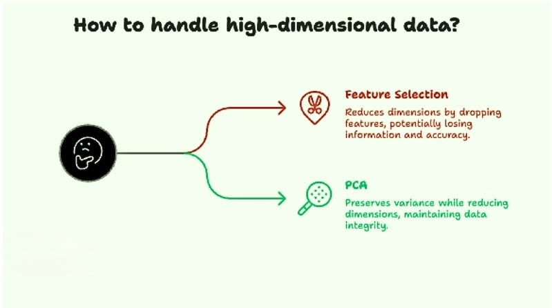
A straightforward solution might be feature selection — simply remove some features and train the model using fewer variables.

but, this approach has a big drawback:

Important information may be lost
Model accuracy may decrease

So instead of discarding features, we need a way to compress information without losing what matters.

This is where Principal Component Analysis (PCA) comes in.

What is PCA

It is an unsupervised algorithm that reduces the number of features (dimensions) in a dataset while preserving as much of the data’s variance as possible.

Why do we need to preserve variance?

1. Variance captures information

· Variance measures how much data varies or spreads out.

· If a feature has zero variance, it carries no information (it’s constant).

· Such features cannot help a model learn patterns.

2. Patterns rely on differences

· Relationships in data are revealed by how variables change relative to each other.

· Without differences (variance), there’s nothing to compare, correlate, or learn from.

3. No variance ⇒ no learning

· If all data points are identical, no model can learn anything meaningful.

This is what the PCA objective is: Basically it applies some transformation to the features to extract new features without loosing the feature importance and by doing so, it minimize the number of features.

In Short:

PCA:

Transforms original features into new features
Retains maximum variance (information)
Reduces the number of dimensions

In Other Words: Reduce dimensions without losing what makes the data informative.

Geometric intuition

Imagine a dataset with with 2 features for simplicity:

House size
Number of rooms
(Target variable: house price — ignored for PCA)

Let’s ignore the target variable. Its goal is only to reduce feature dimensions.

If we were to simply drop “Number of Rooms” (feature selection), we’d lose all variation along that axis. PCA offers a more sophisticated approach.

Let’s analyze the relationship in these 2 features first.

Some relationship between house size and no of rooms

If we project all the data points to both the axes, we will be able to understand the spread of the data which shows the variance of it.

Now our goal is to identify new axes so that a single axis captures the majority of the data’s variance.

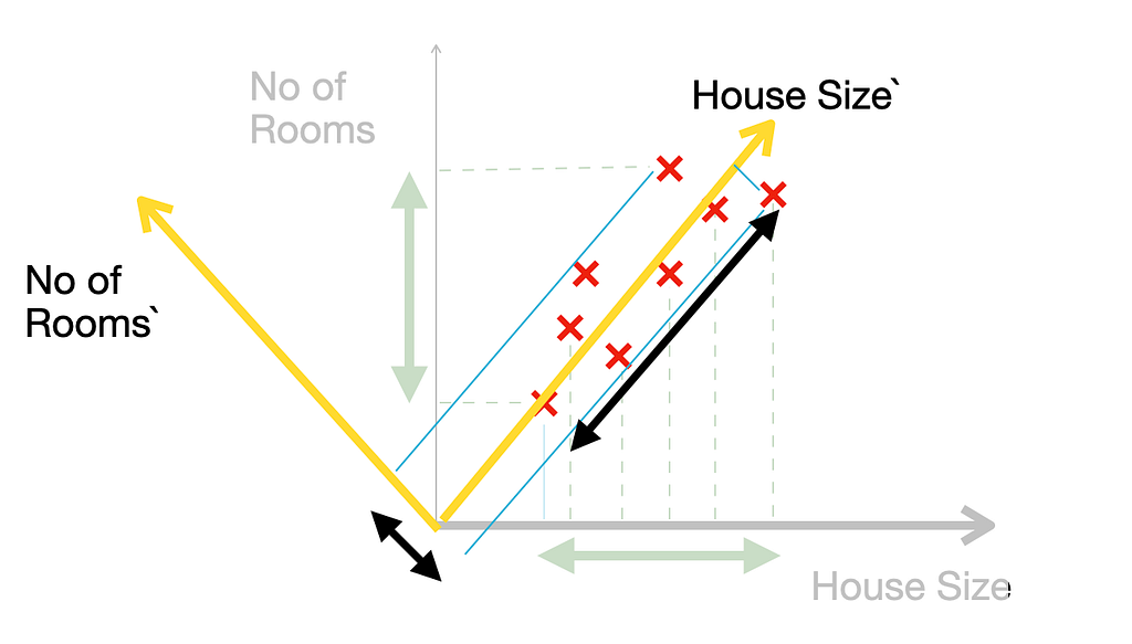
If you notice above, new Size’ axis will capture nearly all the variance of the data. The other axis (No of Rooms’) axis would then become almost insignificant, allowing us to discard it without losing much information.

Remember: this example uses only two features to demonstrate how PCA reduces dimensionality while preserving variance. In practice, PCA is applied to datasets with hundreds of features and compresses them into a smaller set (for example, 10 principal components) that capture the maximum possible variance.

Remember: Idea is to reduce the dimension but still capture the maximum variance.

The new axes created by PCA are called Principal Components:

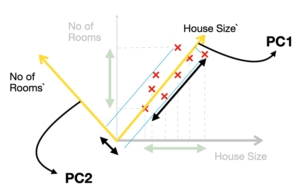
PC1: Captures the maximum variance in the data.
PC2: Captures the second-highest variance and is orthogonal (perpendicular) to PC1.
PC3, PC4, …: For higher dimensions, these capture progressively less variance and are orthogonal to preceding components.

Variance(PC1)>Variance(PC2)>….

If PCA is asked to convert data set from 5D to 3D,

=> It will only consider PC1, PC2 and PC3.

If PCA is asked to convert data set from 5D to 4D,

=> It will only consider PC1, PC2, PC3 and PC4.

How does it work

PCA achieves this dimensionality reduction by performing eigen decomposition on the data’s covariance matrix.

I know this is where things become complicated. Before diving deeper, let’s understand a key concepts and then we’ll come back to this.

Eigen Vector & Eigen Value

Eigenvectors are a fundamental concept in linear algebra, playing a pivotal role in various machine learning and data science applications.

An eigenvector v of a matrix A is a vector that does not change direction when multiplied by A. Mathematically, this is represented as:

Here, lambda is a scalar known as an eigenvalue. This equation tells us that applying the matrix A to the vector x scales the vector by lambda without altering its direction.

Think of it this way: Imagine stretching or rotating a space using a matrix. Most vectors will change their direction. Eigenvectors are the unique vectors that maintain their original direction, only their magnitude changes by a factor of the eigenvalue.

Let me show you through the visualization.

https://medium.com/media/55925d0a8ba49fb96099545fd6826539/href

This is an example where we are trying to apply linear transformation to an vector. While doing this you will notice that the direction and the magnitude changes with the linear transformation.

https://medium.com/media/e9fc64c28f71a342e49112ef7a885747/href

But there will be some vector in this space for a given matrix, on which if we apply this matrix, direction wont change. Only magnitude will change. That is what is called Eigen vector.

In essence:

Eigenvector: The direction of maximum variance.
Eigenvalue: The magnitude of variance along that eigenvector’s direction.

Covariance and Covariance Matrix

A measure of how two variables change together. It gives you only direction, not the strength of the relationship.

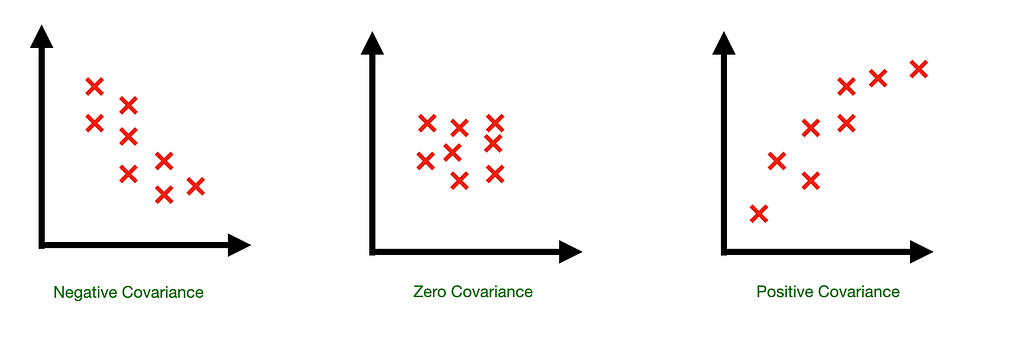
Positive Covariance: Variables tend to increase or decrease together.
Negative Covariance: One variable tends to increase as the other decreases.
Near-Zero Covariance: Little to no linear relationship.

However, covariance alone only tells us direction, not the strength of the relationship. Which means it could be wrong to conclude that there might be a high relationship between variables when the covariance is high.

The Covariance Matrix expands on this by providing a comprehensive view of the spreads(variances) and orientations(covariances) among all pairs of features in a dataset.

It describes how two variables vary together:

Diagonal entries: variances of each variable.
Off-diagonal entries: covariances between pairs of variables (positive if they increase together, negative if one increases while the other decreases).

Covariance matrix for 2 features and 3 features

We only started with 2 dimensional data, but this matrix can be of any size based on the dimension of the data.

How Covariance Matrix, Eigen Vector, Eigen Value, PCA is all related

We now understand what a covariance matrix is and what eigenvectors and eigenvalues are. The question is: how do these concepts work together in PCA?

Remember: PCA starts by examining relationships between features. Next, we reach the point where we want new axes (directions) that let us represent the data in fewer dimensions while still capturing the main patterns. Now think about the covariance matrix. The covariance matrix is a compact way to describe how the data are spread out and how different features co-vary. That means the covariance matrix should help us find these new axes (vectors) that capture the most variance.

ok. we understand covariance matrix can help us but how? A matrix alone doesn’t look like “directions,” so how do we get them? Linear algebra gives us the answer.

This is where mathematician, Karl Pearson, helped us. If we want to represent the covariance matrix with a vector and its magnitude, we need vectors that:

point in the directions of largest spread in the data, and
have magnitudes equal to the spread (variance) in those directions.

Such a vector is an eigenvector, and its magnitude is the corresponding eigenvalue.

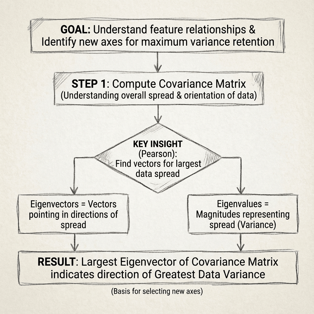
In other words, the largest eigen vector of the covariance matrix always points into the direction of the largest variance of the data.

Perfect — eigenvectors are exactly the new axes PCA seeks, and we can find them from the covariance matrix. In other words: the principal components are the eigenvectors of the data’s covariance matrix.

The second largest eigen vector is always orthogonal to the largest eigenvector, and points into the direction of the second largest spread of data.

A covariance matrix more than 2D will give us multiple eigenvectors having different eigenvalues.

Thus, PCA typically computes principal components by performing eigen-decomposition of the data covariance matrix.

How PCA Works: Step-by-Step

Standardize the Data: Center the data around zero and scale features so that all variables contribute equally.
Calculate the Covariance Matrix: Understand how features vary with respect to each other.
Calculate the Eigenvalues and Eigenvectors: Identify directions of maximum variance using covariance matrix
Sort the Eigenvectors
Project the Data onto the Principal Components: Transform the original data into a lower-dimensional space.

Other than this, PCA helps as a Visualization Aid: By projecting high-dimensional data into a 2D or 3D space using the top principal components, we can visually inspect clusters, outliers, and patterns that would otherwise remain hidden.

Code Example

Conclusion:

PCA is a fundamental technique in data science for several compelling reasons:

Reduces Dimensionality: Makes models more efficient and less prone to the Curse of Dimensionality.
Preserves Information: Retains the most important variance, minimizing information loss.
Improves Model Performance: Faster training and often better generalization due to reduced noise.
Aids Visualization: Unlocks insights by allowing us to see high-dimensional data in lower dimensions.

PCA — Covariance Matrix, Eigen Vector, Eigen value was originally published in Towards AI on Medium, where people are continuing the conversation by highlighting and responding to this story.

Like 0

Liked Liked