
Calculating the expected range of normal samples

The previous post looked at the expected IQ range in a jury of 12. This post will look more generally at computing the expected range of n samples from a N(0, 1) random variable. This will give the expected range in units of σ, i.e. multiply the results by σ if your σ isn’t 1.
As mentioned in the previous post, the expected range is given by

where φ and Φ are the PDF and CDF of a standard normal. The integral can be calculated in closed form for n ≤ 5, but in general it requires numerical integration [1].
The following Python code can compute dn.
from scipy.stats import norm
from scipy.integrate import quad
import numpy as np

def d(n):
    integrand = lambda x: x*norm.pdf(x)*norm.cdf(x)**(n-1)
    res, info = quad(integrand, -np.inf, np.inf)
    return 2*n*res
For large n we have the asymptotic approximation
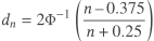
which we could implement in Python by
def approx(n):
    return 2*norm.ppf((n - 0.375)/(n + 0.25))
For very large n the asymptotic expression may be more accurate than the integral due to numerical integration error.
Here are a few example values.
|-----+-------|
|   n |   d_n |
|-----+-------|
|   2 | 1.128 |
|   3 | 1.693 |
|   5 | 2.326 |
|  10 | 3.078 |
|  12 | 3.258 |
|  23 | 3.858 |
|  50 | 4.498 |
| 100 | 5.015 |
|-----+-------|
[1] Order Statistics by H. A. David. John Wiley & Sons. 1970.
The post Calculating the expected range of normal samples first appeared on John D. Cook.
