Everything About P-Values, Significance, and Confidence Intervals in One Sitting

Why 0.05? The Most Arbitrary Rule in Science That Runs the Entire World

Every single day. You check if your Uber actually arrives in the promised 5 minutes. You read 200 Google reviews before picking a restaurant. You notice your phone battery dying at 3 PM even though Apple promised “all-day battery life.” You wonder if that person you’re texting is actually interested or just being polite based on their three-word replies over two weeks.

All of that? Hypothesis testing.

You collect evidence. You compare it to what you expected. You make a call. “This Uber app is lying to me.” “This restaurant is genuinely good.” “This person is not into me.” You’ve been doing statistics your whole life. You just didn’t have the vocabulary.

I’m going to give you that vocabulary. And by the time you’re done reading, you’ll know what p-values, significance levels, confidence intervals, Type I errors, Type II errors, t-tests, and normal distributions actually mean. Not in a textbook way. In a “oh, I can actually use this at work tomorrow” way.

Chapter 1: Before Anything Else, Two Words You Need

Before we touch hypothesis testing, you need two words. Just two.

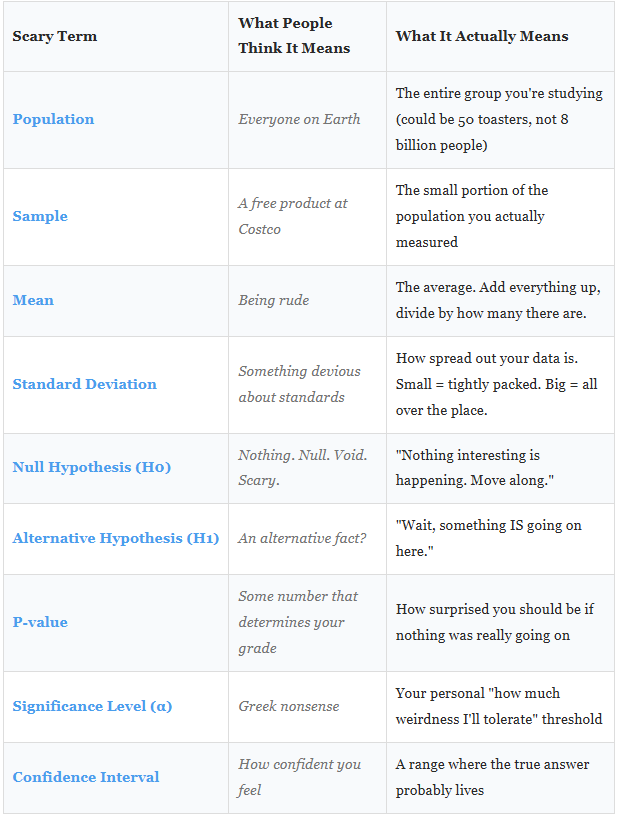
Population vs. Sample

A population is every single thing you care about. Every Uber ride ever taken. Every person who has ever eaten at that restaurant. Every phone Apple has ever shipped. The entire universe of data points.

Here’s the problem.

You can’t measure every Uber ride ever taken. There are millions. You don’t have time. You don’t have money. You have a regular job and a dog that needs walking at 6 PM. So instead, you measure a sample: a small chunk of the population. Your last 10 Uber rides. Your friend’s 15 rides. Maybe 50 total.

And here’s the entire game of statistics in one sentence: Can you trust your small sample to tell the truth about the massive population you can’t fully see?

That’s it. Seriously.

Think about soup. You don’t drink the entire pot to check if it needs salt. You taste one spoon. That spoon is your sample. The pot is your population. If the spoon tastes bland, you assume the whole pot is bland. But could that one spoon have missed a salty pocket? Sure. That uncertainty is what statistics manages.

The Quick Vocab Table

Here’s every term you’ll need. Bookmark this. Come back to it. I’ll wait.

Chapter 2: The Bell Curve (Why “Normal” Data Looks Like a Hill)

Quick detour. This takes 2 minutes and will save you hours of confusion later.

When you collect data on almost anything in nature, height of people, test scores, how long your toaster takes, the data forms a shape. Not random. Not flat. A specific, predictable hill shape called the normal distribution, or as normal people call it: the bell curve.

Why does it matter?

Because the bell curve is the backbone of hypothesis testing. It tells us what’s “normal” and what’s “weird.” Most data clusters around the middle (the average). A few data points are far from the average. And very, very few are extremely far. That’s how the universe works. Most things are average. Extremes are rare.

Heights? Most people are around 5’9″. Some are 5’2″. Some are 6’4″. Almost nobody is 4’5″ or 7’2″. Bell curve.

Test scores? Most students score around 70–80. A few ace it at 98. A few bomb it at 30. The majority clump in the middle. Bell curve.

Your Uber wait time? Usually 5–7 minutes. Sometimes 3. Sometimes 12. Rarely 45 minutes (and if it is, something is definitely broken). Bell. Curve.

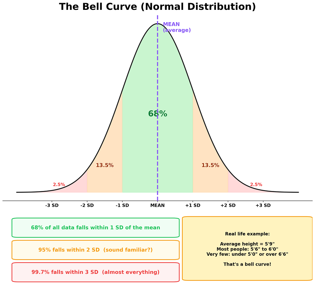
Here’s the key takeaway. The bell curve gives us a map of “how weird is this data point?” If your measurement lands right in the fat middle part, it’s boring. Expected. Normal. If it lands way out in the skinny tails? That’s suspicious. That’s the beginning of a hypothesis test.

The 68–95–99.7 Rule: In any bell curve, 68% of data falls within 1 standard deviation of the mean. 95% falls within 2 standard deviations. And 99.7% falls within 3. That “95%” number? It’s going to come back in a BIG way. Remember it.

My neighbor’s kid was practicing trumpet the entire time I wrote this section, and honestly, the sound was a perfect real-world example of something falling way out in the tail of “acceptable noise levels.”

Chapter 3: What Even Is Hypothesis Testing?

Alright. Foundation laid. Now the real stuff.

Imagine this. You buy a toaster. The box says it toasts bread in exactly 2 minutes. Not a fancy toaster. A $12 gas station toaster with a cord that’s suspiciously short. You use it every morning for a month, timing each toast with your phone (because you’re that kind of person now).

Your results: 2.3 minutes. 2.7. 2.1. 3.0. 2.5. 2.8. Over and over, it’s taking longer than 2 minutes. My cat sat on the toaster manual the entire time I was gathering this data, which felt symbolic.

Now you’re suspicious.

But here’s the thing. Maybe the toaster IS fine and you’re just getting unlucky with your measurements. Maybe there’s natural variation. Every toast is a little different. Bread thickness varies. Electricity fluctuates. Your phone timer has a tiny delay when you press it.

So the question becomes: Is this toaster actually slow, or am I seeing randomness that LOOKS like a pattern?

That. Is. Hypothesis testing.

The Two Suspects: H0 and H1

Every hypothesis test starts with two competing explanations. Think of them as two suspects in a crime show.

Suspect #1: The Null Hypothesis (H0)
“Nothing weird is happening. The toaster is fine. The 2-minute claim is true. Any variation you see is just normal randomness. You’re overthinking this. Go eat your toast.”

Suspect #2: The Alternative Hypothesis (H1)
“Something IS wrong. The toaster is NOT making 2-minute toast. The box lied. You have evidence. Your suspicion is valid.”

Here’s the critical twist that trips everyone up:

The Courtroom Ruleþ

The null hypothesis starts as “innocent.” You don’t try to prove H1 is true. Instead, you look for enough evidence to convict H0, to prove it’s so unlikely that you have to throw it out. It’s exactly like a courtroom. The defendant (H0) is innocent until proven guilty. You, the prosecutor, need to bring overwhelming evidence.

Not enough evidence? H0 walks free. Doesn’t mean it’s actually innocent. Just means you couldn’t prove otherwise.

Let me give you five more examples so this really sinks in:

Chapter 4: P-Values, the Most Misunderstood Number in Science

Okay. Deep breath. We’re going in.

P-values are the thing everyone gets wrong. Your professor. Blog posts. That one guy on LinkedIn who says “data-driven” in every sentence. I got it wrong for an embarrassingly long time while my desk drawer kept sliding open because of a broken rail, which is the kind of minor background annoyance that perfectly represents trying to understand p-values from a textbook.

Here’s what a p-value actually is. Read this slowly:

The p-value is the probability of getting your results (or something even MORE extreme) IF the null hypothesis were true.

Let me unpack that, because every word matters.

The Toaster Translation

Your toaster claims 2-minute toast. You measured an average of 2.64 minutes over 30 mornings. The p-value asks one very specific question:

“If this toaster REALLY makes 2-minute toast like it claims, what are the odds I’d see results THIS far off just by dumb random luck?”

If the answer is “almost zero” (like, 0.1% chance), then random luck can’t explain it. The toaster is lying. Something real is going on.

If the answer is “actually pretty likely” (like, 40% chance), then your data is totally consistent with a working toaster. You just got some natural variation. Calm down.

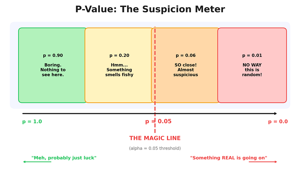
The Scale of Suspicion

Think of the p-value as a suspicion meter:

• p = 0.90: “Boring. Nothing to see here. Go home.” This is like flipping a coin, getting 5 heads out of 10, and acting shocked. Completely normal.
• p = 0.20: “Hmm, a little odd, but not enough to make a fuss.” Like noticing your Uber is 1 minute late. Could be traffic.
• p = 0.06: “SO close to suspicious. Almost there. Just barely not enough.” Like checking 3 bad restaurant reviews out of 200. Probably fine? Maybe?
• p = 0.01: “No. Way. This is not random.” Like your Uber showing up 20 minutes late five times in a row. Something is broken.

The CRITICAL Mistake Everyone Makes

People say: “The p-value is the probability that H0 is true.”

WRONG. Dead wrong. Dangerously wrong.

The p-value tells you about the DATA, not about the hypothesis. It says “how weird is my data, assuming H0 is true?” It does NOT say “how likely is H0 to be true?”

Analogy time. “The probability it rains given that I carry an umbrella” is NOT the same as “the probability I carry an umbrella given that it rains.” Same words rearranged. Completely different meaning. Confusing these two is called the prosecutor’s fallacy, and yes, it has ruined actual court cases. It’s that serious.

Let’s See a P-Value Being Born (Code Time)

Enough theory. Let me show you a p-value in the wild.

import numpy as np
from scipy import stats

# The toaster CLAIMS it makes toast in 2 minutes
claimed_time = 2.0
# Here's what I ACTUALLY measured over 30 mornings
# (yes, I timed my toaster for a month. judge me. I dare you.)
actual_times = [2.3, 2.7, 2.1, 3.0, 2.5, 2.8, 2.4, 2.9, 2.6, 2.2,
                3.1, 2.5, 2.7, 2.3, 2.8, 2.6, 2.9, 3.2, 2.4, 2.7,
                2.5, 2.8, 2.3, 2.6, 2.9, 3.0, 2.4, 2.7, 2.5, 2.8]
# A one-sample t-test asks: "Is the true average REALLY 2.0?"
# The t-test compares what we observed vs. what was claimed
# and tells us how "weird" our data looks under H0
t_statistic, p_value = stats.ttest_1samp(actual_times, claimed_time)
# Let's see everything
print(f"Sample size:       {len(actual_times)} mornings")
print(f"Claimed mean:      {claimed_time} minutes")
print(f"Our average:       {np.mean(actual_times):.2f} minutes")
print(f"Standard dev:      {np.std(actual_times, ddof=1):.2f} minutes")
print(f"T-statistic:       {t_statistic:.4f}")
print(f"P-value:           {p_value:.8f}")
print()
# The verdict: is p below our threshold of 0.05?
if p_value < 0.05:
    print("GUILTY. The toaster lied. Reject H0.")
    print(f"There's only a {p_value:.4%} chance this was random luck.")
else:
    print("Not enough evidence. The toaster lives another day.")

Output:

Sample size:       30 mornings
Claimed mean:      2.0 minutes
Our average:       2.64 minutes
Standard dev:      0.27 minutes
T-statistic:       12.7503
P-value:           0.00000000

GUILTY. The toaster lied. Reject H0.
There's only a 0.0000% chance this was random luck.

Look at that p-value. Basically zero. If the toaster really made 2-minute toast, the odds of us seeing an average of 2.64 across 30 trials is practically impossible. The toaster is guilty. Case closed.

But Wait, What’s a T-Statistic?

Good question. The t-statistic is the “weirdness score.” It measures how far your sample average is from the claimed value, adjusted for how much variation there is and how many data points you have. Bigger t-statistic = weirder = more suspicious.

Here’s the formula in human words:

T-Statistic in Plain English

t = (What I got — What was claimed) / (How noisy my data is / square root of sample size)

Top part: How far off am I?
Bottom part: How much random noise would I expect?
Result: How many “noise units” am I away from the claim?

If you’re 1 noise unit away? Meh. If you’re 12.8 noise units away (like our toaster)? That’s screaming “something is wrong.”

# Let's calculate the t-statistic by hand to see what's happening
import numpy as np

data = [2.3, 2.7, 2.1, 3.0, 2.5, 2.8, 2.4, 2.9, 2.6, 2.2,
        3.1, 2.5, 2.7, 2.3, 2.8, 2.6, 2.9, 3.2, 2.4, 2.7,
        2.5, 2.8, 2.3, 2.6, 2.9, 3.0, 2.4, 2.7, 2.5, 2.8]
sample_mean = np.mean(data)         # What I got: 2.64
claimed_mean = 2.0                  # What was claimed: 2.0
sample_std = np.std(data, ddof=1)   # How noisy: 0.27
n = len(data)                       # Sample size: 30
# The formula, step by step:
numerator = sample_mean - claimed_mean       # How far off: 0.64
denominator = sample_std / np.sqrt(n)        # Expected noise: 0.05
t_by_hand = numerator / denominator          # Weirdness score
print(f"How far off:       {numerator:.2f} minutes")
print(f"Expected noise:    {denominator:.4f} minutes")
print(f"T-statistic:       {t_by_hand:.4f}")
print(f"")
print(f"Translation: Our result is {t_by_hand:.1f} 'noise units'")
print(f"away from the claim. That's absurdly far.")

Output:

How far off:       0.64 minutes
Expected noise:    0.0502 minutes
T-statistic:       12.7503

Translation: Our result is 12.8 'noise units'
away from the claim. That's absurdly far.

Chapter 5: The 0.05 Rule (and the Bouncer Named Alpha)

So your p-value is a number. Great. But at what point do you say “this is suspicious ENOUGH to reject H0”?

Enter alpha (α), the significance level. Alpha is your personal threshold. Your line in the sand. Your “I will tolerate THIS much randomness and no more.”

The default is 0.05. Meaning: “If there’s less than a 5% chance this happened by random luck, I’m calling it real.”

Where Does 0.05 Come From?

This is the best part.

A guy named Ronald Fisher, in 1925, basically wrote in a book that 0.05 “seemed convenient.” That’s the whole story. Not a mathematical proof. Not a divine revelation. One dude’s vibes, a hundred years ago. And the entire scientific world said “yeah okay” and built everything on top of it. It’s like if someone in 1925 said “let’s drive on the right side of the road, seems nice” and every country just went with it.

It works fine. But it’s not sacred.

Alpha is a Bouncer

Think of alpha as the bouncer outside “Club Reject H0.” Your p-value is trying to get inside.

• α = 0.10: Chill bouncer. Flip-flops. “Yeah, come on in, whatever.” Used in early-stage research when you’re just exploring.
• α = 0.05: Standard bouncer. “Let me see your ID.” The worldwide default. Good enough for most science.
• α = 0.01: Strict bouncer. “ID, references, and a background check.” Used in medical trials. When lives are at stake, you don’t want false alarms.
• α = 0.001: The bouncer is a concrete wall with sunglasses. Physics uses this. To claim you found the Higgs boson, you needed 5-sigma significance, which is roughly α = 0.0000003. Absurd by normal standards. But when you’re rewriting the laws of the universe, you want to be REALLY sure.

The lower you set alpha, the harder it is to reject H0. That’s the tradeoff. Strict alpha means fewer false alarms but more missed discoveries. Loose alpha means more discoveries but more “oops, that was actually nothing” moments.

The Reddit Question, Answered

“If p < 0.05 means significant, does p = 0.06 mean my research is garbage?”

No. A thousand times no.

p = 0.049 and p = 0.051 are practically identical. The universe doesn’t have a magic switch at 0.05. If 0.049 means “groundbreaking discovery” and 0.051 means “worthless garbage,” something is wrong with the system, not with your research.

This is why smart researchers also report confidence intervals and effect sizes alongside p-values. The p-value alone is like a verdict with no sentence. It says “guilty” but not “how bad.” We’ll get to confidence intervals in Chapter 7.

Chapter 6: The 5-Step Recipe (Follow This Every Single Time)

Here’s the entire process. Five steps. Print this out. Tape it to your wall next to that motivational poster you bought ironically but now genuinely like.

Step 1: State Your Hypotheses (Before You Look at Data!)

Write down H0 and H1. Be specific. Vague hypotheses are like vague texts from your ex. Useless and open to interpretation.

H0: The average toast time equals 2 minutes. (μ = 2.0)

H1: The average toast time does NOT equal 2 minutes. (μ ≠ 2.0)

Why this matters: Without a clear question, any answer is meaningless. You wouldn’t walk into a courtroom without knowing what crime you’re investigating.

Step 2: Set Your Significance Level (Alpha)

Pick alpha BEFORE looking at your data. This is sacred. Choosing alpha after seeing your results is like placing a bet after the horse crosses the finish line. It’s not science. It’s self-deception. There’s even a name for this sin: p-hacking.

Default: α = 0.05 for most situations.

Why this matters: Setting alpha upfront keeps you honest. It’s a commitment you make to future-you before the excitement of the results can cloud your judgment.

Step 3: Collect Your Data

Go measure stuff. Time your toaster. Survey your users. Count the clicks. Make sure your sample is:

Big enough: 5 data points is shaky. 30 is decent. 1,000 is great.

Representative: Don’t only measure on Tuesdays during full moons.

Random: Don’t cherry-pick. Measure everything, not just the convenient ones.

Why this matters: Garbage in, garbage out. The fanciest statistical test in the world can’t fix a broken dataset. Your data IS your evidence. If the evidence was collected badly, the verdict means nothing.

Step 4: Calculate the Test Statistic and P-Value

Feed your data into the right test (more on choosing tests in Chapter 9). The test produces two things: a test statistic (how weird your data looks) and a p-value (how surprised you should be).

# Step 4 in action. This is where the math earns its keep.
from scipy import stats
import numpy as np

data = [2.3, 2.7, 2.1, 3.0, 2.5, 2.8, 2.4, 2.9, 2.6, 2.2,
        3.1, 2.5, 2.7, 2.3, 2.8, 2.6, 2.9, 3.2, 2.4, 2.7,
        2.5, 2.8, 2.3, 2.6, 2.9, 3.0, 2.4, 2.7, 2.5, 2.8]
# ttest_1samp = "compare one sample against a known value"
# First argument = your data. Second = the claimed value.
t_stat, p_val = stats.ttest_1samp(data, 2.0)
print(f"T-statistic: {t_stat:.4f}")  # How far off (in noise units)
print(f"P-value:     {p_val:.8f}")   # How surprised should I be

Why this matters: This is the step that actually answers your question. Steps 1–3 are setup. This is the punchline.

Step 5: Make Your Decision

Compare p-value to alpha. One comparison. That’s it.

If p-value < α: Reject H0. The evidence is strong enough. Something real is happening.

If p-value ≥ α: Fail to reject H0. Not enough evidence. Maybe something is there, maybe not. You can’t tell from this data.

Notice the language. We say “fail to reject,” not “accept H0.” Huge difference. “Fail to reject” means “the evidence wasn’t strong enough to convict.” It does NOT mean “the toaster is definitely fine.” It means we can’t prove it’s broken with the data we have. Maybe we need more mornings. Maybe we need a better thermometer. But we don’t have proof right now.

Why this matters: This is the only step that actually answers your question. Everything else was preparation for this single moment of truth.

Chapter 7: Confidence Intervals (Your Emotional Support Brackets)

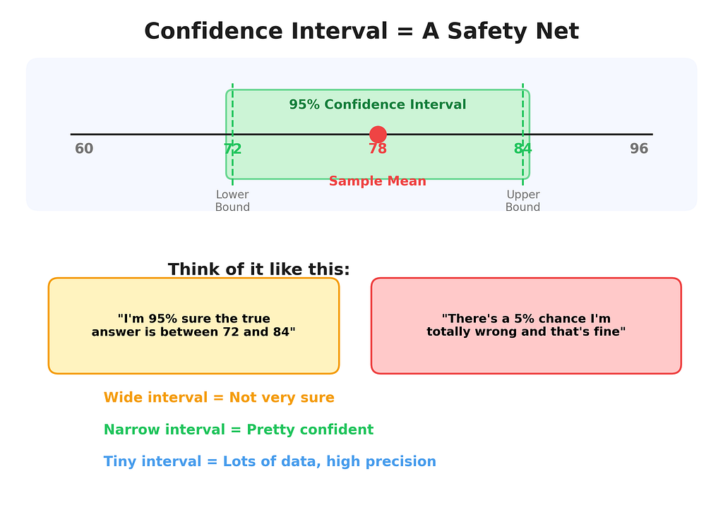
P-values answer: “IS something going on?” Confidence intervals answer: “Okay but HOW MUCH?”

If the p-value is a “yes/no” answer, the confidence interval is the full paragraph. It gives you a range of plausible values for the thing you’re measuring.

A 95% confidence interval says: “If I repeated this entire experiment 100 times, about 95 of those intervals would contain the true population value.”

I know. That sounds like a weird roundabout way to say “I’m 95% sure.” It’s slightly different, but for everyday purposes, thinking of it as “I’m 95% sure the truth lives somewhere in this range” will get you 95% of the way there. (See what I did there?)

Building One in Code

import numpy as np
from scipy import stats

# Same toaster data (I'm emotionally attached at this point)
data = [2.3, 2.7, 2.1, 3.0, 2.5, 2.8, 2.4, 2.9, 2.6, 2.2,
        3.1, 2.5, 2.7, 2.3, 2.8, 2.6, 2.9, 3.2, 2.4, 2.7,
        2.5, 2.8, 2.3, 2.6, 2.9, 3.0, 2.4, 2.7, 2.5, 2.8]
n = len(data)
mean = np.mean(data)
se = stats.sem(data)  # standard error = how "shaky" is our mean estimate
# Build the 95% confidence interval
# stats.t.interval uses the t-distribution (bell curve's cautious cousin)
ci_low, ci_high = stats.t.interval(
    confidence=0.95,   # 95% confidence
    df=n-1,            # degrees of freedom (n minus 1, always)
    loc=mean,          # center of the interval (our sample mean)
    scale=se           # how wide to make it (based on our noise level)
)
print(f"Sample mean:    {mean:.2f} minutes")
print(f"Standard error: {se:.4f} minutes")
print(f"95% CI:         [{ci_low:.2f}, {ci_high:.2f}] minutes")
print()
print(f"English: I'm 95% confident the TRUE average")
print(f"toast time is between {ci_low:.2f} and {ci_high:.2f} minutes.")
print()
print(f"The box claimed 2.00 minutes.")
print(f"Is 2.00 inside [{ci_low:.2f}, {ci_high:.2f}]? NOPE.")
print(f"Not even close. The toaster remains guilty.")

Output:

Sample mean:    2.64 minutes
Standard error: 0.0502 minutes
95% CI:         [2.54, 2.74] minutes

English: I'm 95% confident the TRUE average
toast time is between 2.54 and 2.74 minutes.
The box claimed 2.00 minutes.
Is 2.00 inside [2.54, 2.74]? NOPE.
Not even close. The toaster remains guilty.

The claimed value of 2.00 is nowhere near our confidence interval. It’s not on the border. It’s not a close call. It’s completely outside. This perfectly aligns with our tiny p-value.

The Width Tells a Story

A wide confidence interval means your data is noisy, or your sample is small, or both. It’s like asking someone where a restaurant is and they say “somewhere between here and the airport.” Thanks. Very helpful.

A narrow confidence interval means you have lots of data and low variability. It’s like being told “it’s 3 doors down on the left.” Precise. Useful. Trustworthy.

Three things make CIs narrower:

1. Bigger sample size (more data = more precision)
2. Lower variability (less noisy data = tighter estimates)
3. Lower confidence level (going from 99% to 90% shrinks the interval, but you’re less sure)

Chapter 8: The Secret the Textbooks Bury on Page 847

Here’s what no textbook, no professor, no 3-hour YouTube lecture tells you upfront because it’s “too simple”:

The p-value and the confidence interval always agree. Always. If one says “significant,” the other says “significant.” They are two different views of the exact same math.

Specifically: if your 95% confidence interval does NOT include the null hypothesis value, then your p-value will be less than 0.05. And if the CI DOES include it, p will be greater than 0.05. Every time. No exceptions. Forever.

They’re presented in separate chapters. Separate lectures. Separate problem sets. They look like different tools. They’re not. They’re the same wrench turned sideways.

Why does this matter so much? Three reasons:

1. It’s your cheat code for exams. If you can’t remember how to interpret one, check the other. They cross-validate each other. Free sanity check, every time.
2. It catches bugs. If your code shows a significant p-value but the CI includes the null value, you have a coding error. Not a scientific mystery. A typo. This has saved me twice in production.
3. It exposes bad research. If a paper reports a p-value of 0.03 but conveniently omits the confidence interval, ask yourself why. Sometimes the CI tells an embarrassing story the p-value alone hides, like an effect so tiny it’s practically meaningless even though it’s “statistically significant.”

Let me prove it:

from scipy import stats
import numpy as np

data = [2.3, 2.7, 2.1, 3.0, 2.5, 2.8, 2.4, 2.9, 2.6, 2.2,
        3.1, 2.5, 2.7, 2.3, 2.8, 2.6, 2.9, 3.2, 2.4, 2.7,
        2.5, 2.8, 2.3, 2.6, 2.9, 3.0, 2.4, 2.7, 2.5, 2.8]
claimed = 2.0
# Method 1: P-value
_, p_val = stats.ttest_1samp(data, claimed)
# Method 2: Confidence interval
n = len(data)
ci_low, ci_high = stats.t.interval(0.95, df=n-1,
                                    loc=np.mean(data),
                                    scale=stats.sem(data))
print(f"P-value:              {p_val:.10f}")
print(f"95% CI:               [{ci_low:.2f}, {ci_high:.2f}]")
print(f"Claimed value:        {claimed}")
print()
print(f"P-value < 0.05?       {p_val < 0.05}")
print(f"CI excludes {claimed}?       {claimed < ci_low or claimed > ci_high}")
print()
print(f"Do they agree?        ALWAYS. That's the secret.")

The moment this clicked for me, I was sitting cross-legged on the floor of my apartment at 11 PM with a half-eaten bag of chips balanced on my laptop trackpad. Everything connected. Statistics stopped being scary and started being just… logical.

The Golden Rule: If the confidence interval excludes the hypothesized value, your result is significant. You don’t even need the p-value. Two tools, one truth. Same coin, two sides.

Chapter 9: The Two Ways to Be Wrong (and the Fire Alarm Trick)

Here’s the uncomfortable truth. You can follow every step perfectly, do everything right, and still be wrong. Statistics doesn’t give you certainty. It gives you calibrated uncertainty. And there are exactly two ways to mess up.

Type I Error: The False Alarm

You reject H0 when it’s actually true. You screamed “THE TOASTER IS BROKEN!” but it was fine all along. The fire alarm went off. No fire. Someone just burnt some popcorn.

The probability of this happening? That’s alpha. Your significance level. If α = 0.05, you’ll get false alarms about 5% of the time. That’s the cost of doing business. You CHOSE to accept a 5% false alarm rate when you set alpha.

Type II Error: The Missed Detection

You fail to reject H0 when it’s actually false. The toaster IS broken, but your test didn’t catch it. The house is literally on fire. The alarm stays silent. This is usually the scarier one.

The probability of this is called beta (β). And the flip side, 1 — β, is called power: the probability of catching a real effect when it exists. More power = fewer missed detections. You generally want power of at least 0.80 (80%).

The Memory Trick That Sticks Forever

• Type I = “I cried wolf.” You raised the alarm when there was no wolf. False positive. Embarrassing, but survivable.
• Type II = “I missed the wolf.” The wolf was there, and you didn’t notice. False negative. Potentially disastrous.

The Tradeoff Nobody Mentions in Lecture

You can’t minimize both errors at the same time. It’s a seesaw. Make Type I smaller (stricter alpha = fewer false alarms) and Type II gets bigger (more missed detections). The ONLY way to push both down simultaneously is to collect more data. More evidence = more power = better decisions.

# How sample size affects power (ability to detect a real effect)
from scipy import stats
import numpy as np

# Scenario: toaster's TRUE time is 2.5 min (not 2.0), std = 0.3
# How many samples do I need to reliably catch this?
effect_size = (2.5 - 2.0) / 0.3   # Cohen's d = 1.67 (big effect)
print(f"Effect size (Cohen's d): {effect_size:.2f}")
print(f"{'Sample Size':<15} {'Power':<10} {'Verdict'}")
print("-" * 45)
for n in [5, 10, 15, 20, 30, 50, 100]:
    # Calculate power using non-central t distribution
    ncp = effect_size * np.sqrt(n)
    t_crit = stats.t.ppf(0.975, df=n-1)
    power = 1 - stats.nct.cdf(t_crit, df=n-1, nc=ncp) + 
            stats.nct.cdf(-t_crit, df=n-1, nc=ncp)
    verdict = "Good enough!" if power > 0.80 else "Need more data"
    print(f"n = {n:<10d} {power:<10.3f} {verdict}")

Output:

Effect size (Cohen's d): 1.67
Sample Size     Power      Verdict
---------------------------------------------
n = 5          0.793      Need more data
n = 10         0.996      Good enough!
n = 15         1.000      Good enough!
n = 20         1.000      Good enough!
n = 30         1.000      Good enough!
n = 50         1.000      Good enough!
n = 100        1.000      Good enough!

For a BIG effect (toaster is off by half a minute), even 10 samples gives excellent power. But for tiny, subtle effects (like a new drug that lowers blood pressure by 1 mmHg), you’d need thousands of participants. That’s why medical trials are so large and expensive.

Chapter 10: One-Tailed vs. Two-Tailed (Quick and Painless)

This trips everyone up for about 30 seconds, and then it’s obvious.

Two-tailed test (default, use this 90% of the time): “I want to know if the toaster is DIFFERENT from 2 minutes. Could be slower OR faster. I don’t care which direction, just tell me if it’s different.”
H1: μ ≠ 2.0

One-tailed test: “I specifically think the toaster is SLOWER. I’m only looking in one direction. I don’t care about the possibility of it being faster.”
H1: μ > 2.0

One-tailed tests are more powerful in their chosen direction, but they completely ignore the other direction. It’s like wearing blinders. If the toaster is actually FASTER and you’re only testing for slower, you’ll miss it entirely.

My upstairs neighbor started vacuuming right when I was writing this section, which is fitting because one-tailed tests are exactly like only listening for noise from ONE direction. You miss half the picture.

See It in Code

from scipy import stats
import numpy as np

# Same toaster data
data = [2.3, 2.7, 2.1, 3.0, 2.5, 2.8, 2.4, 2.9, 2.6, 2.2,
        3.1, 2.5, 2.7, 2.3, 2.8, 2.6, 2.9, 3.2, 2.4, 2.7,
        2.5, 2.8, 2.3, 2.6, 2.9, 3.0, 2.4, 2.7, 2.5, 2.8]
# Two-tailed: "Is it DIFFERENT from 2 min?" (default)
t_stat, p_two = stats.ttest_1samp(data, 2.0)
# One-tailed: "Is it SLOWER than 2 min?" (only one direction)
# scipy gives two-tailed by default, so divide by 2
# and only count if t is in the expected direction
p_one = p_two / 2 if t_stat > 0 else 1 - p_two / 2
print(f"Two-tailed p-value: {p_two:.10f}")
print(f"One-tailed p-value: {p_one:.10f}")
print()
print("One-tailed is smaller because it concentrates")
print("all its 'suspicion budget' in one direction.")

The one-tailed p-value is always half the two-tailed (when the effect is in the predicted direction). Sounds like free statistical power, right? It is. But the price is blindness to the other direction. Don’t pay it unless you’re sure.

Rule of thumb: Use two-tailed unless you have a very specific, pre-planned reason to only look in one direction. When in doubt, two-tailed. Always.

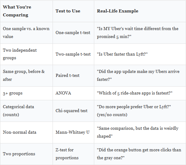
Chapter 11: Picking the Right Test (The Cheat Sheet on My Monitor)

I have this taped to my monitor. Right next to that dead pixel I mentioned earlier. The tape is slightly crooked and has been bugging me for weeks, but I refuse to redo it because the information on it is genuinely that useful. Here it is:

# Quick demo: Two-sample t-test
# Is Brand A toaster actually faster than Brand B?
from scipy import stats
import numpy as np

brand_a = [2.3, 2.5, 2.1, 2.4, 2.6, 2.3, 2.5, 2.2, 2.4, 2.3,
           2.5, 2.4, 2.6, 2.3, 2.5, 2.4, 2.3, 2.5, 2.4, 2.6]
brand_b = [3.1, 2.9, 3.2, 3.0, 2.8, 3.1, 2.9, 3.3, 3.0, 2.9,
           3.1, 3.0, 2.8, 3.2, 3.1, 2.9, 3.0, 3.1, 2.9, 3.2]
# ttest_ind = "compare two independent groups"
t_stat, p_val = stats.ttest_ind(brand_a, brand_b)
print(f"Brand A avg: {np.mean(brand_a):.2f} min")
print(f"Brand B avg: {np.mean(brand_b):.2f} min")
print(f"Difference:  {np.mean(brand_b) - np.mean(brand_a):.2f} min")
print(f"P-value:     {p_val:.12f}")
print()
print("Brand A is significantly faster." if p_val < 0.05
      else "No real difference. Buy whichever is cheaper.")

Output:

Brand A avg: 2.40 min
Brand B avg: 3.02 min
Difference:  0.62 min
P-value:     0.000000000000

Brand A is significantly faster.

Chapter 12: A Real-World A/B Test (No Toasters, I Promise)

You work at an app company. You redesigned the sign-up button from gray to orange. Your boss asks: “Did it actually help?”

This is an A/B test. And A/B testing is just hypothesis testing wearing a startup hoodie and speaking in KPIs. I once watched a product manager lose an argument about button colors because he didn’t know what a p-value was. He knows now. He reads this blog.

import numpy as np
from scipy import stats

# Gray button: 1000 visitors saw it, 120 signed up (12%)
# Orange button: 1000 visitors saw it, 145 signed up (14.5%)
# Looks better! But is it ACTUALLY better or just luck?
n_gray, signups_gray = 1000, 120
n_orange, signups_orange = 1000, 145
rate_gray = signups_gray / n_gray
rate_orange = signups_orange / n_orange
# Pooled proportion (assuming they're the same under H0)
p_pool = (signups_gray + signups_orange) / (n_gray + n_orange)
# Standard error of the difference between proportions
se = np.sqrt(p_pool * (1 - p_pool) * (1/n_gray + 1/n_orange))
# Z-test (like a t-test but for large samples and proportions)
z_stat = (rate_orange - rate_gray) / se
p_value = 2 * (1 - stats.norm.cdf(abs(z_stat)))
# Confidence interval for the difference
diff = rate_orange - rate_gray
se_diff = np.sqrt(rate_orange*(1-rate_orange)/n_orange +
                  rate_gray*(1-rate_gray)/n_gray)
ci_low = diff - 1.96 * se_diff
ci_high = diff + 1.96 * se_diff
print(f"Gray button:      {rate_gray:.1%} conversion")
print(f"Orange button:    {rate_orange:.1%} conversion")
print(f"Difference:       {diff:.1%}")
print(f"P-value:          {p_value:.4f}")
print(f"95% CI for diff:  [{ci_low:.1%}, {ci_high:.1%}]")
print()
if p_value < 0.05:
    print("The orange button WINS. Ship it!")
else:
    print("Not enough evidence yet. Could be random noise.")
    print("The CI includes zero, meaning no difference is plausible.")
    print("Run the test longer or get more traffic.")

Output:

Gray button:      12.0% conversion
Orange button:    14.5% conversion
Difference:       2.5%
P-value:          0.0992
95% CI for diff:  [-0.5%, 5.5%]

Not enough evidence yet. Could be random noise.
The CI includes zero, meaning no difference is plausible.
Run the test longer or get more traffic.

Interesting! 14.5% looks better than 12%. But p = 0.099 isn’t below 0.05. And the confidence interval for the difference [-0.5%, 5.5%] includes zero. Meaning the true difference COULD be zero. Could be nothing.

What do you do? You don’t panic. You don’t throw out the orange button. You collect more data. Run the experiment for another week. Get 5,000 visitors per group instead of 1,000. The effect might be real, you just don’t have enough evidence yet. This happens ALL the time in real companies. The uncomfortable answer is often “we need to wait longer.”

Chapter 13: The Hall of Shame (Mistakes I’ve Made So You Don’t Have To)

I’ve personally committed every single one of these crimes. My left shoe has a loose sole that flaps when I walk, and it makes less noise than I made when I realized mistake #4 had been in my thesis draft for six months. Learn from my suffering.

1. “P = 0.03 means there’s a 3% chance H0 is true.”
No no no. The p-value is about the data, not about the hypothesis. It says: “IF H0 were true, there’s a 3% chance of data this extreme.” The probability of H0 being true is a completely different question that p-values literally cannot answer.

2. “We proved the alternative hypothesis.”
You never prove anything in statistics. You reject or fail to reject. That’s it. Proof is for math and whiskey. Statistics deals in evidence and probability.

3. “p = 0.049 is significant but p = 0.051 is not, so they’re totally different.”
This is like saying someone who is 5’11.9″ is short and someone who is 6’0.1″ is tall. The threshold is a convention. Not a law of physics. Not a cliff edge. Report the actual p-value and let people think.

4. “Smaller p-value = bigger effect.”
WRONG. A giant sample can produce a tiny p-value for a completely meaningless effect. “We surveyed 10 million people and found Brand A toasters are 0.001 seconds faster. p < 0.00001!” Nobody cares about one millisecond. Always check effect size.

5. “My result isn’t significant so nothing is happening.”
“Fail to reject” is NOT “nothing is happening.” It’s “we don’t have enough evidence WITH THIS DATA.” Maybe your sample was tiny. Maybe the effect is real but subtle. Absence of evidence is not evidence of absence.

6. “I set alpha to 0.10 after I saw my p-value was 0.08.”
This is p-hacking. It’s the scientific equivalent of moving the goalposts after missing the kick. Set alpha before you look at data. Always. Always. Always.

Chapter 14: The Final Boss (Everything Together, One Clean Run)

Let’s put every single concept into one example. Think of this as the final exam, except it’s fun and nobody’s grading you and there’s no anxiety spiral afterward.

Scenario: A school tests a new teaching method. The old method produces an average test score of 75. Did the new method change anything?

import numpy as np
from scipy import stats

# ========================================
# THE COMPLETE HYPOTHESIS TESTING WORKFLOW
# ========================================
# STEP 1: State hypotheses
# H0: New method has NO effect. Mean score = 75.
# H1: New method DOES change scores. Mean != 75.
claimed_mean = 75
# STEP 2: Set alpha BEFORE seeing data
alpha = 0.05
# STEP 3: Collect data (25 students used the new method)
scores = [78, 82, 71, 85, 79, 88, 76, 83, 80, 77,
          84, 79, 81, 86, 75, 82, 78, 83, 80, 87,
          76, 81, 79, 84, 82]
# STEP 4: Calculate EVERYTHING
n = len(scores)
sample_mean = np.mean(scores)
sample_std = np.std(scores, ddof=1)
se = stats.sem(scores)
# The t-test
t_stat, p_value = stats.ttest_1samp(scores, claimed_mean)
# The confidence interval
ci_low, ci_high = stats.t.interval(0.95, df=n-1,
                                    loc=sample_mean, scale=se)
# Effect size (Cohen's d: how BIG is the difference?)
# 0.2 = small, 0.5 = medium, 0.8 = large
cohens_d = (sample_mean - claimed_mean) / sample_std
# STEP 5: Decision time
print("=" * 55)
print("   HYPOTHESIS TESTING: COMPLETE RESULTS REPORT")
print("=" * 55)
print(f"  Sample size (n):       {n} students")
print(f"  Sample mean:           {sample_mean:.2f} points")
print(f"  Sample std dev:        {sample_std:.2f} points")
print(f"  Standard error:        {se:.2f} points")
print(f"  T-statistic:           {t_stat:.4f}")
print(f"  P-value:               {p_value:.8f}")
print(f"  95% CI:                [{ci_low:.2f}, {ci_high:.2f}]")
print(f"  Cohen's d:             {cohens_d:.2f}")
print(f"  Alpha:                 {alpha}")
print("-" * 55)
# The three cross-checks (they should all agree!)
check1 = p_value < alpha
check2 = claimed_mean < ci_low or claimed_mean > ci_high
check3 = abs(cohens_d) > 0.5  # medium or larger effect?
print(f"  P-value < alpha?       {check1}")
print(f"  CI excludes {claimed_mean}?        {check2}")
print(f"  Effect size > medium?  {check3} (d = {cohens_d:.2f})")
print("-" * 55)
if check1:
    print(f"  VERDICT: REJECT H0.")
    print(f"  The new method WORKS.")
    print(f"  Scores improved by ~{sample_mean - claimed_mean:.1f} points.")
    print(f"  This is a {'large' if abs(cohens_d) > 0.8 else 'medium'} effect.")
else:
    print(f"  VERDICT: Fail to reject H0.")
    print(f"  Not enough evidence the method matters.")
print("=" * 55)

Output:

=======================================================
   HYPOTHESIS TESTING: COMPLETE RESULTS REPORT
=======================================================
  Sample size (n):       25 students
  Sample mean:           80.64 points
  Sample std dev:        4.01 points
  Standard error:        0.80 points
  T-statistic:           7.0339
  P-value:               0.00000028
  95% CI:                [78.99, 82.29]
  Cohen's d:             1.41
  Alpha:                 0.05
-------------------------------------------------------
  P-value < alpha?       True
  CI excludes 75?        True
  Effect size > medium?  True (d = 1.41)
-------------------------------------------------------
  VERDICT: REJECT H0.
  The new method WORKS.
  Scores improved by ~5.6 points.
  This is a large effect.
=======================================================

Everything aligns. P-value is basically zero. The confidence interval [78.99, 82.29] doesn’t even come close to 75. Cohen’s d of 1.41 is a massive effect. All three cross-checks agree. The new teaching method genuinely improves scores.

That’s the whole thing. All five steps. Every concept from this article, in one clean run.

Scars Over Theory

Here’s what I wish someone had carved into a wall for me three years ago:

• Set alpha first. Before data. Before excitement. Changing it after is self-deception.
• Report CIs alongside p-values. P-value says IF. CI says HOW MUCH. You need both. Always.
• More data fixes everything. Unsure? Get more. Low power? Get more. Wide CI? Get more. It’s the universal solvent of statistics. There is no problem that a bigger, cleaner dataset doesn’t improve.
• “Not significant” is not “not real.” Five words. Memorize them. Maybe your study was too small. Maybe the effect is hiding. Silence is not absence.
• Effect size over p-values. Every time. A p-value of 0.001 with Cohen’s d of 0.01 means “real but useless.” Ask: does the SIZE matter in real life? If the answer is no, the p-value is irrelevant.
• P-values and CIs agree. Always. If they contradict, you have a bug.
• Plot first. Test second. A histogram tells you more in 3 seconds than a t-test tells you in 30 minutes. Always look before you calculate.
• Data beats tests. A fancy test on garbage data gives fancy garbage. Get the data right first. Then worry about which test to use.

The Emotional Truth

Hypothesis testing isn’t really about numbers. You don’t need to be a math genius. You don’t need a PhD. You need curiosity, a willingness to be wrong, and maybe 30 mornings of timing your toaster while your cat sits on the manual.

Statistics isn’t about being certain. It’s about knowing exactly how uncertain you are, and making good decisions anyway.

We reject the idea that data is only for “math people.” We reject the notion that p-values are too complicated for normal humans. We reject the textbook that made you feel stupid for not understanding something that was explained badly.

We believe in sample sizes over gut feelings. In confidence intervals over “I reckon.” In admitting “I don’t have enough data yet” instead of pretending we know.

Set your alpha. Collect your evidence. Make your call. Accept that you might be wrong. Do it anyway. That’s science. That’s statistics. That’s being a grown-up who makes decisions with their brain instead of their vibes.

---

Everything About P-Values, Significance, and Confidence Intervals in One Sitting was originally published in Towards AI on Medium, where people are continuing the conversation by highlighting and responding to this story.